PPO

[[On-Policy & Off-Policy]] → near on policy

• sample reuse

创新点 → [[Importance Sampling]] 和 clip 机制

• 在策略优化过程中，与环境交互的策略（旧策略）与要更新的策略（新策略）不同。所以需要 → 能够从一个分布中采样可以估计另一个分布。
• 用重要性采样来估计 → 策略梯度
  • 由于采样轨迹的分布与当前策略分布之间的差异会导致 → 梯度估计的偏差
    • 通过 {{c1 比率因子}} 校正偏差，以更准确地估计策略梯度

[[Policy Gradient]] $g=\nabla J(\theta)=E_{a^{\sim} \pi(\theta)}\left[Q_{\pi(\theta)}\left(S_t, a_t\right) \nabla \log \pi_\theta\right]$

• 利用策略 $\pi^{\prime}$ 代为采样，转化 → [[Off-Policy]]
  • 梯度 → $g=\nabla J(\theta)=E_{a^{\sim} \pi(\theta)^{\prime}}\left[\frac{\pi(\theta)}{\pi(\theta)^{\prime}} Q_{\pi(\theta)^{\prime}}\left(S_t, a_t\right) \nabla \log \pi_\theta\right]$
• PPO 修复引入 PG 后的重要性采样不足
  • 方法 → 每步收益会比期望的收益好多少，也就是advantage
  • 梯度 → $g=E_{a^{-} \pi(\theta)}\left[A_{\pi(\theta)}\left(s_t, a_t\right) \nabla \log \pi_\theta\right]$
• 合并重要性采样和 advantage function 后的梯度 #card
  • $g=E_{a^{\sim} \pi(\theta)^{\prime}}\left[\frac{\pi(\theta)}{\pi(\theta)^{\prime}} A_{\pi(\theta)^{\prime}}\left(s_t, a_t\right) \nabla \log \pi_\theta\right]$
    • $\pi_\theta \nabla \log \pi_\theta=\nabla \pi_\theta$ → $g=E_{a^{\sim} \pi(\theta)^{\prime}}\left[\frac{\nabla \pi(\theta)}{\pi(\theta)^{\prime}} A_{\pi(\theta)^{\prime}}\left(s_t, a_t\right)\right]$
• PPO 对应的目标函数 → $J(\theta)^{\prime}=E_{a^{\sim} \pi(\theta)^{\prime}}\left[\frac{\pi(\theta)}{\pi(\theta)^{\prime}} A_{\pi(\theta)^{\prime}}\left(s_t, a_t\right)\right]$

为了克服 {{c2 采样的分布与原分布差距过大的不足}}，PPO 引入 {{c1 KL 散度}} 进行约束。

• 公式变成 → $J(\theta)^{\prime}=E_{a^{\sim} \pi(\theta)^{\prime}}\left[\frac{\pi(\theta)}{\pi(\theta)^{\prime}} A_{\pi(\theta)^{\prime}}\left(s_t, a_t\right)\right]-\beta K L\left(\pi(\theta)^{\prime}, \pi(\theta)\right)$ KL距离做正则
• [[TRPO]](Trust Region Policy Optimization)，要求 $K L\left(\theta, \theta^{\prime}\right)<\delta$
• 实际应用中基于采样估计期望，省略 KL 距离的计算，对应的目标函数 #card
  • $J(\theta)^{\prime} \approx \sum_{(s, a)} \min \left(\frac{\pi(\theta)}{\pi(\theta)^{\prime}} A_{\pi(\theta)^{\prime}}, \operatorname{clip}\left(\frac{\pi(\theta)}{\pi(\theta)^{\prime}}, 1-\varepsilon, 1+\varepsilon\right) A_{\pi(\theta)^{\prime}}\right)$

引入 KL 散度和 clip 分解解决什么问题？#card

• KL 散度解决新旧分布差异
• clip 解决前后策略差异

PPO Loss → $L^{C L I P}(\theta)=\hat{\mathbb{E}}_t\left[\min \left(r_t(\theta) \hat{A}_t, \operatorname{clip}\left(r_t(\theta), 1-\epsilon, 1+\epsilon\right) \hat{A}_t\right)\right]$

• Ratio Function 算计公式 → $r_t(\theta)=\frac{\pi_\theta\left(a_t \mid s_t\right)}{\pi_{\theta_{\text {old }}}\left(a_t \mid s_t\right)}$
  • ratio function denotes the probability ratio between {{c1 the current and old policy}}
    • If $r_t(\theta)>1$, → the action $a_t$ at state $s_t$ is more likely in the current policy than the old policy.
    • If $r_t(\theta)$ is between 0 and 1 → the action is less likely for the current policy than for the old one.
• The unclipped part → $L^{C P I}(\theta)=\hat{\mathbb{E}}t\left[\frac{\pi\theta\left(a_t \mid s_t\right)}{\pi_{\theta_{\text {old }}}\left(a_t \mid s_t\right)} \hat{A}_t\right]=\hat{\mathbb{E}}_t\left[r_t(\theta) \hat{A}_t\right]$
• The clipped Part → $\operatorname{clip}\left(r_t(\theta), 1-\epsilon, 1+\epsilon\right) \hat{A}_t$
  • 论文限制范围 0.8 到 1.2
• $\hat{A}_t$ 是 {{c1 优势估计函数}}，PPO 原始论文使用 {{c1 [[generalized advantage estimation]]}}
• we take the minimum of the clipped and non-clipped objective, so the final objective is a {{c1 lower bound (pessimistic bound)}} of the unclipped objective.
  • Taking the minimum of the clipped and non-clipped objective means we’ll select either the clipped or the non-clipped objective based on {{c1 the ratio and advantage situation.}}

限制两次更新之间有过大的策略更新

• TRPO (Trust Region Policy Optimization) uses {{c1 KL divergence}} constraints outside the objective function to constrain the policy update. But this method is complicated to implement and takes more computation time.
• PPO {{c1 clip probability ratio directly}} in the objective function with its Clipped surrogate objective function.

((66dd2f00-54d1-4fbd-a04c-8e4a699c19e0))

• $1-\varepsilon \leq \operatorname{clip}\left(\frac{\pi(\theta)}{\pi(\theta)^{\prime}}, 1-\varepsilon, 1+\varepsilon\right) \leq 1+\varepsilon$
  • $A_{\pi(\theta)^{\prime}}>0$ → 当前策略表现好，需要增大 $\pi( \theta )$
    • $\min \left(\frac{\pi(\theta)}{\pi(\theta)^{\prime}} A_{\pi(\theta)^{\prime}}, \operatorname{clip}\left(\frac{\pi(\theta)}{\pi(\theta)^{\prime}}, 1-\varepsilon, 1+\varepsilon\right) A_{\pi(\theta)^{\prime}}^{\prime}\right)$ 得 $\frac{\pi(\theta)}{\pi(\theta)^{\prime}} \leq 1+\varepsilon$
      • 通过 clip 增加参数更新的上下限防止 → 新旧分布相差太大，引入误差
  • $A_{\pi(\theta)^{\prime}}<0$ → 当前策略表现差
    • $\min \left(\frac{\pi(\theta)}{\pi(\theta)^{\prime}} A_{\pi(\theta)^{\prime}}, \operatorname{clip}\left(\frac{\pi(\theta)}{\pi(\theta)^{\prime}}, 1-\varepsilon, 1+\varepsilon\right) A_{\pi(\theta)^{\prime}}^{\prime}\right)$ 得 $\frac{\pi(\theta)}{\pi\left(\theta \theta^{\prime}\right.} \geq 1-\varepsilon$
      • clip 限制下限 → 需要大幅度改变 $\pi( \theta )

[[CLIP]] 控制 → 策略更新的幅度

• 限制 $r_t(\theta)$ 更新范围在→ $[1-\epsilon, 1+\epsilon]$
• 作用 → 有助于保持算法的稳定性，并避免在单次更新中引入过大的策略变化。
  

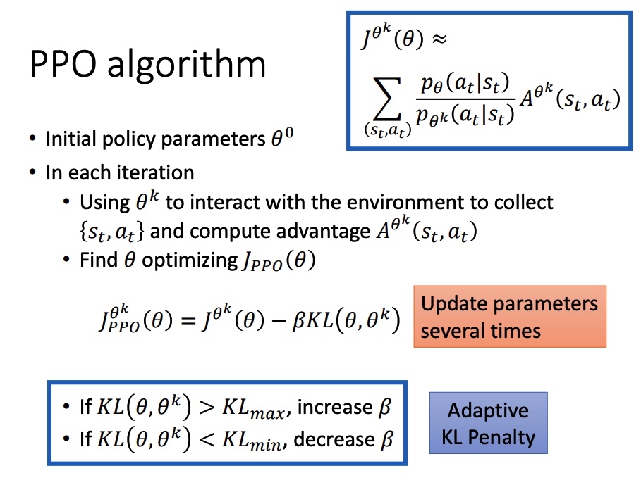
[[PPO]] algorithm

• 系数 $\beta$ 在迭代的过程中需要进行动态调整。引入 $KL_{max} KL_{min}$，KL > KLmax，说明 penalty 没有发挥作用，增大 $\beta$。
  • 若当前的KL距离比最大KL距离还大, 说明采样分布与更新的分布距离更大了, 表示约束还不够强力，需要 $\beta$ 增大；
  • 反之, 若当前的KL距离比最小的KL距离还小, 则 $\beta$ 缩小。
    

[[Ref]]

• 强化学习之PPO - 知乎 (zhihu.com)
• 【点滴】策略梯度之PPO - 知乎 (zhihu.com)

网络回响