@Informer: Beyond Efficient Transformer for Long Sequence Time-Series Forecasting

[[Abstract]]

  • Many real-world applications require the prediction of long sequence time-series, such as electricity consumption planning. Long sequence time-series forecasting (LSTF) demands a high prediction capacity of the model, which is the ability to capture precise long-range dependency coupling between output and input efficiently. Recent studies have shown the potential of Transformer to increase the prediction capacity. However, there are several severe issues with Transformer that prevent it from being directly applicable to LSTF, including quadratic time complexity, high memory usage, and inherent limitation of the encoder-decoder architecture. To address these issues, we design an efficient transformer-based model for LSTF, named Informer, with three distinctive characteristics: (i) a ProbSparse self-attention mechanism, which achieves O(L log L) in time complexity and memory usage, and has comparable performance on sequences’ dependency alignment. (ii) the self-attention distilling highlights dominating attention by halving cascading layer input, and efficiently handles extreme long input sequences. (iii) the generative style decoder, while conceptually simple, predicts the long time-series sequences at one forward operation rather than a step-by-step way, which drastically improves the inference speed of long-sequence predictions. Extensive experiments on four large-scale datasets demonstrate that Informer significantly outperforms existing methods and provides a new solution to the LSTF problem.

[[Attachments]]

Long sequence [[Time Series Forecasting]] (LSTF)

  • 长序列时间序列预测需要模型能够有效捕捉输出和输入之间精确的 long-range dependency coupling

LSTF 中使用 [[Transformer]] 需要解决的问题 #card #incremental

  • self-attention 计算复杂度 O(L2)O(L^2)

  • 多层 encoder/decoder 结构内存增长

  • dynamic decoding 方式预测耗时长

网络结构

ProbSparse self-attention

  • 替换 inner product self-attention

    • [[Sparse Transformer]] 结合行输入和列输出

    • [[LogSparse Transformer]] cyclical pattern

    • [[Reformer]] locally-sensitive hashing(LSH) self-attention

    • [[Linformer]]

    • [[Transformer-XL]] [[Compressive Transformer]] use auxiliary hidden states to capture long-range dependency

    • [[Longformer]]

  • 其他优化 self-attention 工作存在的问题

    • 缺少理论分析

    • 对于 multi-head self-attention 每个 head 都采用相同的优化策略

  • self-attention 点积结果服从 long tail distribution

    • 较少点积对贡献绝大部分的注意力得分

    • 现实含义:序列中某个元素一般只会和少数几个元素具有较高的相似性/关联性

  • 第 i 个 query 用 qiq_i 表示

    • A(qi,K,V)=jf(qi,kj)lf(qi,kl)vj=Ep(kjqi)[vj]\mathcal{A}\left(q_i, K, V\right)=\sum_j \frac{f\left(q_i, k_j\right)}{\sum_l f\left(q_i, k_l\right)} v_j=\mathbb{E}_{p\left(k_j \mid q_i\right)}\left[v_j\right]

    • p(kjqi)=k(qi,kj)lf(qi,kl)p\left(k_j \mid q_i\right)=\frac{k\left(q_i, k_j\right)}{\sum_l f\left(q_i, k_l\right)}

    • k(qi,kj)=exp(qikjTd)k\left(q_i, k_j\right)=\exp \left(\frac{q_i k_j^T}{\sqrt{d}}\right)

  • query 稀疏性判断方法

    • p(kjqj)p(k_j|q_j)[[均匀分布]] q 的 [[KL Divergence]]

      • q 是均分分布,相等于每个 key 的概率都是 1L\frac{1}{L}

      • 如果 query 得到的分布类似于均匀分布,每个概率值都趋近于 1L\frac{1}{L},值很小,这样的 query 不会提供什么价值。

      • p 和 q 分布差异越大的结果越是我们需要的 query
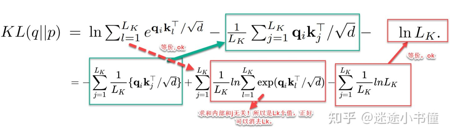
      • p 和 q 的顺序和论文中的不同 D(pq)=xp(x)logp(x)q(x)=Ep(x)(logp(x)q(x))D(p \| q)=\sum_{x} p(x) \log \frac{p(x)}{q(x)}=E_{p(x)}\left(\log \frac{p(x)}{q(x)}\right)

    • KL(qp)=lnl=1LkeqiklT/d1Lkj=1LqikjT/dlnLkK L(q \| p)=\ln \sum_{l=1}^{L_k} e^{q_i k_l^T / \sqrt{d}}-\frac{1}{L_k} \sum_{j=1}^L q_i k_j^T / \sqrt{d}-\ln L_k

      • 把公式代入,然后化解

+ $M\left(q_i, K\right)=\ln \sum_{l=1}^{L_k} e^{q_i k_l^T / \sqrt{d}}-\frac{1}{L_k} \sum_{j=1}^{L_k} q_i k_j^T / \sqrt{d}$

  + 第一项是经典难题 log-sum-exp(LSE) 问题

  + 稀疏性度量 $M\left(q_i, K\right)$

    + $\ln L \leq M\left(q_i, K\right) \leq \max _j\left\{\frac{q_i k_j^T}{\sqrt{d}}\right\}-\frac{1}{L} \sum_{j=1}^L\left\{\frac{q_i k_j^T}{\sqrt{d}}\right\}+\ln L$

    + LSE 项用最大值来替代,即用和当前 qi 最近的 kj,所以才有下面取 top N 操作

      + $\bar{M}\left(\mathbf{q}_i, \mathbf{K}\right)=\max _j\left\{\frac{\mathbf{q}_i \mathbf{k}_j^{\top}}{\sqrt{d}}\right\}-\frac{1}{L_K} \sum_{j=1}^{L_K} \frac{\mathbf{q}_i \mathbf{k}_j^{\top}}{\sqrt{d}}$

+ $\mathcal{A}(\mathbf{Q}, \mathbf{K}, \mathbf{V})=\operatorname{Softmax}\left(\frac{\overline{\mathbf{Q}} \mathbf{K}^{\top}}{\sqrt{d}}\right) \mathbf{V}$

  + $\bar{Q}$ 是稀疏矩阵,前 u 个有值

+ 具体流程

  + 为每个 query 都随机采样 N 个 key,默认值是 5lnL

    + 利用点积结果服从长尾分布的假设,计算每个  query 稀疏性得分时,只需要和采样出的部分 key 计算

  + 计算每个 query 的稀疏性得分

  + 选择稀疏性分数最高的 N 个 query,N 默认值是 5lnL

  + 只计算 N 个 query 和所有 key 的点积结果,进而得到 attention 结果

  + 其余 L-N 个 query 不计算,直接将 self-attention 层输入取均值(mean(V))作为输出

    + 除了选中的 N 个query index 对应位置上的输出不同,其他 L-N 个 embedding 都是相同的。所以新的结果存在一部分冗余信息,也是下一步可以使用 maxpooling 的原因

    + 保证每个 ProbSparse self-attention 层的输入和输出序列长度都是 L

+ 将时间和空间复杂度降为 $$O(L_K \log L_Q)$$

+ 如何解决 对于 multi-head self-attention 每个 head 都采用相同的优化策略

现象?

  + 每个 query 随机采样 key 这一步每个 head 的采样结果是相同的

  + 每一层 self-attention 都会先对 QKV 做线性转换,序列中同一个位置不同 head 对应的 query、key 向量不同

  + 最终每个 head 中得到的 N 个稀疏性最高的 query 也是不同的,相当于每个 head 都采取不同的优化策略

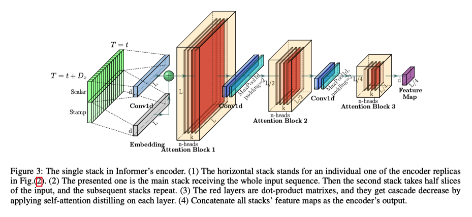
Self-attention distilling

  • 突出 dominating score,缩短每一层输入的长度,降低空间复杂度到 O((2ϵ)LlogL)\mathcal{O}((2-\epsilon) L \log L)

  • encoder 层数加深,序列中每个位置的输出已经包含序列中其他元素的信息,所以可以缩短输入序列的长度

    • 过 attention 层后,大部分位置值相同
  • 激活函数 [[ELU]]

  • 通过 Conv1d + max-pooling layer 缩短序列长度

1
2
3
4
5
6
7
8
9
10
11
12
13
14
15
16
17
18
19
class ConvLayer(nn.Module):
def __init__(self, c_in):
super(ConvLayer, self).__init__()
self.downConv = nn.Conv1d(in_channels=c_in,
out_channels=c_in,
kernel_size=3,
padding=2,
padding_mode='circular')
self.norm = nn.BatchNorm1d(c_in)
self.activation = nn.ELU()
self.maxPool = nn.MaxPool1d(kernel_size=3, stride=2, padding=1)

def forward(self, x):
x = self.downConv(x.permute(0, 2, 1))
x = self.norm(x)
x = self.activation(x)
x = self.maxPool(x)
x = x.transpose(1,2)
return x

Generative style decoder

  • 预测阶段通过一次前向得到全部预测结果,避免 dynamic decoding

  • 不论训练还是预测,Decoder 的输入序列分成两部分 Xfeeddcoder=concat(Xtoken,Xplaceholder)X_{feed dcoder} = concat(X_{token}, X_{placeholder})

    • 预测时间点前一段已知序列作为 start token

    • 待预测序列的 placeholder 序列

  • 经过 deocder 后,每个 placeholder 都有一个向量,然后输入到一个全链接层得到预测结果

  • 为什么用 generative style decoder #card

    • 解码器能捕捉任意位置输出和长序列依赖关系

    • 避免累积误差

Experiment

  • Baseline

  • 实验设计

    • Univariate Time-series Forecasting

    • Multivariate Time-series Forecasting

      • LSTnet 是基线模型
    • Ablation Study

Input representation

  • 提供时序信息

  • 不是天级别更新的模型需要 global time stamp

    • week,month,holiday embedding
  • 额外实验

    • 利用 t0-t1 的特征预测 t2-t3 结果还不错

    • 可能是 local time stamp 和 global time stamp 让 informer 不依赖自回归结果还能有不错的预测结果

See Also

Ref


@Applying Deep Learning To Airbnb Search

[[Abstract]]

  • The application to search ranking is one of the biggest machine learning success stories at Airbnb. Much of the initial gains were driven by a gradient boosted decision tree model. The gains, however, plateaued over time. This paper discusses the work done in applying neural networks in an attempt to break out of that plateau. We present our perspective not with the intention of pushing the frontier of new modeling techniques. Instead, ours is a story of the elements we found useful in applying neural networks to a real life product. Deep learning was steep learning for us. To other teams embarking on similar journeys, we hope an account of our struggles and triumphs will provide some useful pointers. Bon voyage!

[[Attachments]]

记录 Airbnb 深度模型探索历程。

业务:顾客查询后返回一个有序的列表(Listing,对应房间)。

深度模型之前使用 GBDT 对房子进行打分。

Model Evolution

  • 评价指标 [[NDCG]]

  • Simple NN

    • 32 层 NN + Relu,特征和优化目标和 GBDT 效果相同

    • 打通深度模型训练和线上预测的 pipeline。

  • LambdaRank NN

    • [[LambdaRank]] 直接优化 NDCG

    • 采用 pairwise 的训练方式,构造 <被预定的房间,未被预定的房间> 的训练样本

    • pairwise loss 乘上 item 对调顺序带来的指标变化 NDCG,关注列表中靠前位置的样本

      • 比如 booked listing 从 2 到 1 的价值比 books listing 从 10 到 9 的意义大。
  • Decision Tree/Factorization Machine NN

+ GBDT 叶子节点位置(类别特征) + FM 预测结果放到 NN 中。
  • Deep NN

    • 10 倍训练数据,195 个特征(离散特征 embedding 化),两层神经网络:127 fc + relu 以及 83 fc + relu。

    • 部分 dnn 的特征是来自其他模型,之间在 [[@Real-time Personalization using Embeddings for Search Ranking at Airbnb]] 里面提到的特征也有使用。

    • 在训练样本达到 17 亿后,ndcg 在测试集和训练集的表现一致,这样一来可以使用线下的效果来评估线上的效果?

    • 深度模型在图像分类任务上已经超过人类的表现,但是很难判断是否在搜索任务上也超过人类。一个关键是很难定义搜索任务中的人类能力。

Failed Models

  • Listing ID

    • listing id 进行 embedding,但是出现过拟合。

      • embedding 需要每个物品拥有大量数据进行训练,来挖掘他们的价值

      • 部分 Listing 有一些独特的属性,需要一定量的数据进行训练。

  • Multi-task learning

    • booking 比 view 更加稀疏,long view 和 booking 是有相关的。

    • 两个任务 Booking Logit 和 Long View Logit,共享网络结构。两个指标在数量级上有差异,为了更加关注 booking 的指标,long view label 乘上 log(view_duration)。

      • 线上实验中,页面浏览的时间提高,但是 booking 指标基本不变。

      • 作者分析长时间浏览一个页面可能是高档房源或页面描述比较长。

  • [[Feature Engineering]]

    • GBDT 常用的特征工程方法:计算比值,滑动窗口平均以及特征组合。

    • NN 可以通过隐层自动进行特征交叉,对特征进行一定程度上的处理可以让 NN 更加有效。

  • Feature [[Normalization]]

    • NN 对数值特征敏感,如果输入的特征过大,反向传播时梯度会很大。

    • 正态分布

    • (featurevalμ)/ρ(feature_val - \mu)/\rho

    • power law distribution

    • log1+featureval1+median\log \frac{1+feature_val}{1+median}

  • Feature distribution

    • 特征分布平滑

    • 是否存在异常值?

    • 更容易泛化,保证高层输出有良好的分布

  • [[Hyperparameters]]

    • [[Dropout]] 看成是一种数据增强的方法,模拟了数据中会出现随机缺失值的情况。drop 之后可能会导致样本不再成立,分散模型注意力的无效场景。

      • 替代方案,根据特征分布人工产生噪音加入训练样本,线下有效果,线上没有效果。
    • [[神经网络参数全部初始化为0]] 没有效果,[[Xavier Initialization]] 初始化参数,Embedding 使用 -1 到 1 的随机分布。

    • Learning rate 默认参数 [[Adam]] 效果不太好,使用 [[LazyAdam]] 在较大 embedding 场景下训练速度更快

  • Feature Importance [[可解释性]]

    • Score Decomposition 将 NN 的分数分解到特征上。[[GBDT]] 可以这样做。

    • Ablation Test 每次训练一个模型删除一个特征。问题是模型可以从剩余的特征中弥补出缺失的特征。

    • Permutation Test 选定一个特征,随机生成值。[[Random Forests]] 中常用的方法。新生成的样本可能和现实世界中的分布不同。一个特征可能和其他特征共同作用产生效果。

    • TopBot Analysis 分析排序结果 top 和 bot 的单独特征分布

      • 左边代表房子价格的分布,top 和 bot 的分布存在明显不同,代表模型对价格敏感。

      • 右边代表页面浏览量的分布,top 和 bot 的分布接近,说明模型没有很好利用这个特征。

奇怪的东西

  • 论文中一直在引用 [[Andrej Karpathy]] 的建议:don’t be a hero

@Item2Vec: Neural Item Embedding for Collaborative Filtering

[[Abstract]]

  • Many Collaborative Filtering (CF) algorithms are item-based in the sense that they analyze item-item relations in order to produce item similarities.

  • Recently, several works in the field of Natural Language Processing (NLP) suggested to learn a latent representation of words using neural embedding algorithms. Among them, the Skip-gram with Negative Sampling (SGNS), also known as [[word2vec]], was shown to provide state-of-the-art results on various linguistics tasks.

  • In this paper, we show that item-based CF can be cast in the same framework of neural word embedding.

    • Inspired by SGNS, we describe a method we name item2vec for item-based CF that produces embedding for items in a latent space.

    • The method is capable of inferring item-item relations even when user information is not available.

  • We present experimental results that demonstrate the effectiveness of the item2vec method and show it is competitive with SVD.

[[向量化召回统一建模框架]] 理解 #card

  • nce_loss

image.png