核心贡献
- Temporal Fusion Transformer 框架 #card
- ((6428093d-c9dc-487f-8840-9b7a43376502))
- ((64280946-0abb-40ac-b6b9-7a83c10ed74e))
- ((6428096f-ea71-4205-a89f-1d718e53255e))
- ((64280981-cfd3-47e7-afa8-e8c839f949f7))
- 模型可解释性 ((6428091b-78f2-4d1b-8e87-f83d0953e693)) #card
- 区分全局重要特征 ((64284111-cae0-4a63-a822-bc047e99b95b))
- 持久的时间模式 ((64284147-5c0d-4d47-b4b0-aadfd7737b6f))
- 显著事件 ((64284159-ab32-4882-9c0e-a3a34cd643d4))
核心问题
- [[Multi-horizon Forecasting]] 包含复杂的输入特征组合 ((642807a6-6348-4f39-b439-a891603d2a58)) #card
- 静态变量
- 与时间无关的静态变量 ((642807f6-54d8-4ca5-888e-d35261d7cee6))
- 时变变量 Time-dependent Inputs
- 已知未来输入 ((64280800-1dd7-43af-9fa1-6f25847d003b))
- 外生时间序列 ((6428080d-b6f1-490d-bc32-faf89b228644))
- 历史顾客流量 ((64280a80-2be7-489e-9b49-923eaaf0ef30))
- 相关示意图
- ((642809ea-81f1-46a6-aad5-ed0bff26e75e))
- 使用 attention 机制增强 → 选择过去相关特征 ((64280ad6-b21a-499b-83cc-7ddc6c890a3f))
- 之前基于 DNN 方法的缺陷 #card
- 没有考虑不同类型输入特征 ((64283e4e-a40e-4a44-993f-bc934ecef477))
- 万物皆时序 构建模型时,将所有的特征按 time step 直接 concat 在一起,所有变量全部扩展到所有的时间步,无论是静态、动态的变量都合并在一起送入模型。
- 假定所有外生输入都已知与未来 ((64283e5b-8387-464c-81af-527aa4542538))
- 忽略重要的静态协变量 ((64283e84-bd1d-45d2-886a-0df596a16137))
- 已有深度学习方法是黑箱,如何解释模型的预测结果?#card
- ((642808d2-0b60-4b5f-bf20-b6bb1a790c01))
相关工作
- [[@A Multi-Horizon Quantile Recurrent Forecaster]] Multi-horizon Quantile Recurrent Forecaster MQRNN 结构,同时预测未来多个时间步的值
- deep state space 状态空间模型,统计学,hybrid network,类似工作 [[ESRNN]] [[N-BEATS]]
- [[Explainable AI]]
- post-hoc methods 事后方法(因果方法),不考虑输入特征的时间顺序 ((64283f9d-dfcb-4263-a527-546ea1fc58e4))
- 基于 attention 的架构对语言或语音序列有很好的解释,但是很难适用于多维度预测 ((64284031-ae1a-4815-8137-f599ecbbdaaf))
解决方法
- [[Multi-horizon Forecasting]]
- prediction intervals [[区间预测]] #card
- [[DeepAR]] 直接修改模型的输出,模型不拟合原始标签,而是拟合人工指定的分布,通过蒙特卡洛采样取平均得到最终的点预测。
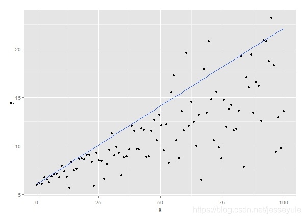
- 分位数回归 [[Quantile Regression]],每一个 time step 输出 $10^{th}$ $50^{th}$ $90^{th}$ #card
- 不同分位数下预测能够产生预测区间,通过区间大小反应预测结果的不确定性。某个点在不同分位数线性回归的预测结果很接近,则预测确定性搞。
- Quantile Outputs
- $\hat{y}i(q, t, \tau)=f_q\left(\tau, y{i, t-k: t}, \boldsymbol{z}{i, t-k: t}, \boldsymbol{x}{i, t-k: t+\tau}, \boldsymbol{s}_i\right)$
- 设计 [[quantile loss]]
- $\begin{gathered}\mathcal{L}(\Omega, \boldsymbol{W})=\sum_{y_t \in \Omega} \sum_{q \in \mathcal{Q}} \sum_{\tau=1}^{\tau_{\max }} \frac{Q L\left(y_t, \hat{y}(q, t-\tau, \tau), q\right)}{M \tau_{\max }} \end{gathered}$
- $Q L(y, \hat{y}, q)=q(y-\hat{y}){+}+(1-q)(\hat{y}-y){+}$ #card
- q 代表分位数
- $()_+ = \max (0,)$
- 假设拟合分位数 0.9
+ $Q L(y, \hat{y}, q=0.9)=\max (0.9 *(y-\hat{y}), 0.1 *(\hat{y}-y))$
+ $y-\hat{y} \gt 0$ 模型预测偏小,Loss 增加更多
+ loss 中权重 9:1,模型倾向预测出大的数字,Loss 下降快
+ 假设拟合分位数 0.5,退化成 MAE
+ $Q L(y, \hat{y}, q=0.5)=\max (0.5 *(y-\hat{y}), 0.5 (\hat{y}-y)) = 0.5|y-\hat{y}|$
+ q-Risk 避免不同预测点下的预测量纲不一致问题,对结果做正则化处理。目前只关注 P50 和 P90 两个分位数 #card
+ $q$-Risk $=\frac{2 \sum_{y_t \in \tilde{\Omega}} \sum_{\tau=1}^{\tau_{\max }} Q L\left(y_t, \hat{y}(q, t-\tau, \tau), q\right)}{\sum_{y_t \in \tilde{\Omega}} \sum_{\tau=1}^{\tau_{\max }}\left|y_t\right|}$
- 模型结构
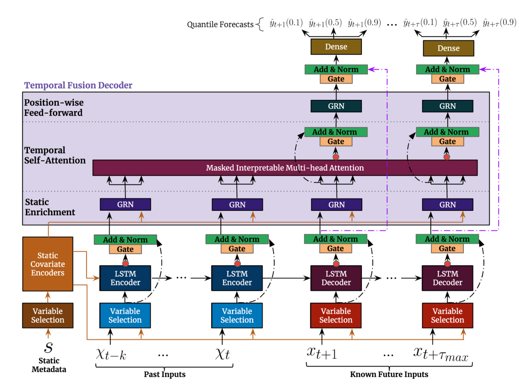
- ((642845bf-6e28-467a-8c0a-5b4e84f34c2c))
- 输入部分
- [[Static Covariate Encoders]] 通过 {{c1 GRN}} 将静态特征编码变成 4 个不同向量
- 动态特征 #card
- post inputs
- known future inputs
- [[Variable Selection Networks]] 通过选择重要的特征,减少不必要的噪音输入,以提供模型性能。#card
- [[GLU]] 灵感来自 LSTM 的门控机制,sigmoid 取值范围 0-1
- 对不同类型的输入变量应该区别对待 #card
- 静态变量通过特殊的 [[Static Covariate Encoders]],后续做为 encoder 和 decoder 的输入
- 过去的动态时变变量+动态时不变变量进入 encoder 结构中(蓝色 variable seletcion)
- 未来的动态时不变变量进入 decoder 结构中
- seq2seq with teacher forcing 架构 #card
- encoder 部分动态特征 embedding 和静态特征 embedding concat 在一起做为输入
- decoder
- 模型组成
- [[Gated Residual Network]] 模型能够灵活地仅在需要时应用非线性处理 #card
- 外生输入和目标之间的确切关系通常是事先未知的,因此很难预见那些变量是相关的。
- 很难确定非线性处理的程度该多大,并且可能存在更简单的模型就能满足需求。
- [[Interpretable Multi-Head Attention]]
- [[Temporal Fusion Decoder]] 学习数据集中的时间关系
- 通过 dense 层得到多个 [[Quantile Outputs]] #card
- $\hat{y}(q, t, \tau)=\boldsymbol{W}_q \tilde{\boldsymbol{\psi}}(t, \tau)+b_q$
[[TFT Interpretability Use Cases]] #card
- 输入特征重要性 ((643eb0f7-d9cc-4b51-992a-aea215af0d68))
- 可视化当前时间模式 ((643eb151-fc5d-491c-b690-d6b7f19fd93c))
- 识别导致任何导致时间动态显著变化的时间 ((643eb1bc-a6a5-4342-9611-83aa4e249d6b))
[[Ref]]