什么是 PS ？

• 分布式进行梯度下降的计算完成参数的更新与最终收敛
• 和 [[Spark MLib]] 一样数据并行训练产生局部梯度，再汇总梯度更新参数权重的并行化训练方案

参数服务面临的挑战

• 访问参数需要的大量带宽
• 算法需要有序更新参数，不同服务器之间同步带来的时延
• 训练容灾

PS 重要特征

• 异步同行
• 灵活的一致性模型
• 弹性扩展
• 容灾
• 方便使用

并行梯度下降流程

• 任务管理器
  • 分发数据到 workder
• Worker
  • 初始化
    • 加载训练数据
    • 从 server 节点拉取参数
  • 迭代
    • 根据本节点训练数据计算梯度
    • 将计算好的梯度 push 到 servers 节点
    • pull 最新需要用到的参数
  • Servers
    • 汇总 m 个 worker 计算出的梯度成总梯度
    • 利用总梯度和正则化项梯度，计算新参数
      

物理架构

• server group 管理，每个 server 维护部分参数
  • 支持自定义梯度更新方式
• Range Push 和 Pull
  • 小批量更新参数
    

一致性和并行效率之间的取舍

• 同步阻断式
  • 等 master 汇总全部梯度，重新计算模型新参数后才开始下一轮计算
• 异步非阻断式
  • 每一轮更新没有关联
• 最大延迟
  • 新的参数没有获取到时，使用旧的参数计算梯度
  • 指定 X 轮迭代必须等待更新参数

Vector Clock

• 记录每个 worker 每个 range 对应的参数时间

多 server 节点的协同和效率问题

• ((7627aee6-0ca0-40b7-a649-0ed86482eb01))
  • 通过[[一致性哈希]]计算参数位置以及分配对应的服务器
  • 服务器 S1 会计算 S1 对应的参数，也会备份之后几个 server 对应的参数
  • 增加节点相当于将 range 分裂
  • 删除节点可以让临近节点负责
    
• server 在汇总多个 workder 的结果之后广播

总结

• 用异步非阻断式的分布式梯度下降策略代替同步阻断式的梯度下降策略
• 实现多 server 节点的架构，避免单 master 节点带来的带宽瓶颈和内存瓶颈
• 使用[[一致性哈希]]，range pull 和 range push 等工程手段实现信息的最小传递，避免广播操作带辣的全局性网络阻塞和带宽浪费

问题

• 各 worker 之间如何同步？
  +
• 如何解决 DNN weight
  • AllReduce 完成 dnn weight 在各 worker 节点同步
  • feature embedding 使用纯异步 ASP 模式，dnn weight 使用纯同步 SSP 模式

worker 之间的并行策略

• BSP（Bulk Synchronous Parallel） #card
  
  
• SSP（Stalness Synchronous Parallel） #card
  
  
• ASP（Asynchronous Parallel） #card
  

实现

• 基于ps-lite实现分布式算法
• 阿里巴巴的XDL
• 快手的Persia

Ref

• 一文读懂「Parameter Server」的分布式机器学习训练原理 - 知乎 (zhihu.com)
• 重温经典之ps-lite源码解析(1)：基础 - 知乎 (zhihu.com)

[[@BERT: Pre-training of Deep Bidirectional Transformers for Language Understanding]]

代码：google-research/bert: TensorFlow code and pre-trained models for BERT

大模型 + 微调提升小任务的效果

输入层

BERT

两种 NLP 预训练

[[ELMo]]

[[GPT]]

贡献性

模型输入：

训练方式

• [[Masked-Language Modeling]] →mask 部分单词，80 % mask，10 % 错误单词， 10% 正确单词
  • 目的 → 训练模型记忆句子之间的关系。
    • 减轻预训练和 fine-tune 目标不一致给模型带来的影响
• [[Next Sentence Prediction]] → 预测是不是下一个句子
  • 句子 A 和句子 B 有 50% 的概率是上下文
  • 解决后续什么问题 → QA 和自然语言推理
    

[[激活函数]] [[GELU]]

优化器

fine tune

研究取不同的 embedding 效果

缺陷

[[Ref]]

• [[Multimodal BERT]]
• The Illustrated BERT, ELMo, and co. (How NLP Cracked Transfer Learning) – Jay Alammar – Visualizing machine learning one concept at a time
• 如何评价 BERT 模型？ - 知乎
• NLP 从语言模型看Bert的善变与GPT的坚守 - 知乎
  • 像Bert这样的双向语言模型为何要做 masked LM？[[GPT]] 为何一直坚持单向语言模型？ Elmo 也号称双向，为何不需要 mask？[[Word2Vec]] 的 CBOW 为何也不用 mask？
  • indirectly see themselves
  • GPT 保留用上文生成下文的能力
• 为什么 Bert 的三个 Embedding 可以进行相加？ - 知乎
  • 三个 embedding 相加和拼接
    • 联系 → 三个 embedding 相加相当于三个原始的 one-hot 拼接再经过一个全连接网络。
      • 优点 → 和拼接相比，相加可以节约模型参数。
      • 实验显示拼接并没有相加效果好，拼接后维度增加，需要再经过一个线性变换降低维度，增加了更多参数。
  • 之前的理解和多个波长不同的波相加，最后还是能分离出来，所以模型也应该能区分。
  • 空间维度很高，模型能区分各个组分
    • 参数空间量 30k2512
    • 模型表达能力至少是 2^768
  • 梯度角度，(f + g +h)' = f' + g' + h'
• BERT—容易被忽视的细节
  • 细节三：对于任务一，对于在数据中随机选择 15% 的标记，其中80%被换位[mask]，10%不变、10%随机替换其他单词，原因是什么？#card
    • [mask] 在 fine-tune 任务中不会出现，模型不知道如何处理。
    • 缓解上面的现象
    • 15% 标记被预测，需要更多训练步骤来收敛

{:height 198, :width 509}

• TCN 中输入和输出可能有不同的宽度，c 图表示使用 11 卷积调整输入大小
  • 也可以直接通过 zero padding 来增加 channels

TCN = 1D FCN + causal convolutions

特点

• 使用因果卷积，不会泄漏未来信息。
  • 论文中强调和 RNN 之类方法进行对比，所以要考虑因果。
• 可以取任意长度的序列，并将其映射到相同长度的输出序列。
• 引入 [[ResNet]] 和扩张卷积的组合可以将网络做深以及增加感受野。

细节

• tcn 中没有 pooling 层
• normalization 方法是 weight norm，更适合序列问题

增加感受野的方法

• 更大的 kernel_size (增加参数，卷积核大效果差，卷积核过大会退化成一个全连接层)
• [[空洞卷积]]

时序问题

• 1. 输入和输出矩阵大小相同
• 2. 不能使用没有发生时刻的信息，因果卷积

[[ETA 模型]] 实现

• ((f431b69d-e38f-4a1f-ac98-1c80d3e0bcbe))

Summary

• 填补 CV 领域有监督学习和无监督学习的差距

Abstract

• dictionary look-up
  • 提出基于队列+动量对比用于无监督的表征学习。

Introduction

• 创新点：用队列表示字典
  • 什么样的字典才适合对比学习？
    • (i) large
      • 从连续高维空间做更多的采样，字典 key 越多，表示的信息越丰富
      • 字典小，key 少，模型泛化能力弱
    • (ii) consistent
      • 字典中的 key 应该用相同或相似的编码器生成
      • 如果key是使用不同编码器得到的，查询时可能找到与 query 使用相同或相似编码器生成的key，而不是语义上相似的 key
• 无监督在 CV 领域不成功的原因
  • 原始信号空间的不同
  • NLP 原始信号是离散的，词、词根、词缀，容易构建 tokenized dictionaries 做无监督学习
    • tokenized: 把一个词对应成某一个特征
    • Why tokenized dictionaries 有助于无监督学习？
    • 把字典的 key 认为是一个类别，有类似标签的信息帮助学习
    • NLP 无监督学习很容易建模，建好的模型也好优化
  • CV 原始信号是连续的、高维的，不像单词具有浓缩好的、简洁的语义信息，不适合构建一个字典
  • 如果没有字典，无监督学习很难建模
• 无监督学习主要的两个部分：
  • pretext tasks 代理任务
    • 学习更好的特征表示
    • 常见代理任务
      • denoising auto-encoders 重建整张图
      • context auto-encoders 重建某个 patch
      • cross-channel auto-encoders (colorization) 给图片上色当自监督信号
      • pseudo-labels 图片生成伪标签
      • exemplar image 给同一张图片做不同的数据增广，它们都属于同一个类。
      • patch ordering 九宫格方法：打乱了以后预测 patch 的顺序, or 随机选一个 patch 预测方位 eight positions
      • 利用视频的顺序做 tracking
      • 做聚类的方法 clustering features
  • loss functions
    • 衡量模型预测结果和固定目标的差异
    • L1 or L2 Loss
      • Auto-encoder
    • 判别式网络
      • eight position
        • 图片 9 等分，判断选出的图片位于中间图片的什么方向。
    • 对比学习损失：目标不固定，训练过程中不断改变
    • 对抗学习损失：衡量两个概率分布之间的差异

Method

• 代理任务 instance discrimination 个体判别
  
  • 一张图片 $$x_{i}$$ 经过翻转+裁剪等方法得到 $$x_{i1}$$ 和 $$x_{i2}$$，这两张图片做为正样本，其他图片做为负样本。
  • $$x_{i1}$$ 是 anchor
  • $$x_{i2}$$ 是 positive
  • 编码器 E11 和 E12 可以相同，也可以不同。
  • 对比学习怎么做？
    • f11 和 f12 接近，和其他样本远离
      • matching key and dissimilar to others
      • Learning is formulated as minimizing a contrastive loss
    • f11 当成是 query，在字典中查询接近的 key
• 如何构建大 + 一致的字典
  
  • 基于队列的字典
    • 摆脱 batch size 的限制
    • 用队列大小限制字典大小
  • 基于动量的编码器
    • $$\theta_{\mathrm{k}} \leftarrow m \theta_{\mathrm{k}}+(1-m) \theta_{\mathrm{q}}$$
    • momentum encoder 由当前的编码器初始化得到
    • 动量 m=0.999 比较大是，动量编码器更新缓慢。尽可能保证队列的 key 由相似的编码器生成
• 和之前方法对比
  • end-to-end 牺牲大
    • 负样本大小等于 batch size 大小
  • memory-bank 牺牲一致性
    • 采样得到负样本
  • moco
    • encoder 基于梯度更新
    • momentum encoder 基于 encoder 进行动量更新
      
• 目标函数 [[InfoNCE]]
  • $$\mathcal{L}{q}=-\log \frac{\exp \left(q \cdot k{+} / \tau\right)}{\sum_{i=0}^{K} \exp \left(q \cdot k_{i} / \tau\right)}$$
  • 计算 q 和 k 的点积判断两个样本之间的相似度
  • $$\tau$$ 控制分布图形，越大越关注困难样本
• 同一张图片的增强版本分别做为两个编码器的输入
  

Experiments

• 7 个检测 + 分割任务
• linear protocol
  • 预训练模型，应用时只改变最后的全连接层。
  • backbone 做为特征提取器
  • 对比预训练的效果好不好

Conclusion

• 1000 倍数据增加，moco 性能提升不高
• 尝试NLP中其他代理任务 masked auto-encoding
  • [[Masked-Language Modeling]]
  • 见 [[Masked Autoencoders Are Scalable Vision Learners]]
• 总结
  • 去构造一个大的字典，从而让正负样本能够更有效地去对比，提供一个稳定的自监督信号，最后去训练这个模型

QR hashing (Shi et al., 2019) offers a solution by decomposing large matrices into smaller ones using quotient and remainder techniques while preserving embedding uniqueness across IDs. 通过使用商数和余数技术将大矩阵分解为较小的矩阵，同时保持不同 ID 嵌入的唯一性 #card

• 减少 embedding 词表大小和通过MurmurHash 这样的抗冲突哈希函数消除词表维护需求

非静态词汇哈希范式示例 Example of non static vocab hashing paradigm #card

• id hash 成一个 quotient 和一个 remainder
  
• 具体流程
  

在 Wide & Deep 基础上，对 Wide 部分进行改进。LR 无法进行特征交叉，FM 受限于性能一般只去做二阶交叉，Cross 可以实现高阶交叉。DCN 和 DNN 相比，相同效果情况下可以减少参数量。

Cross 网络只能处理定长的输入，[[ETA]] v4 中无法使用……

特征处理和常规的模型一样，Sparse feature 经过 embedding 处理，然后和 Dense feature concat 在一起。由于 Cross network 每一层的大小都和输入向量大小相等，如果 Sparse feature 不处理，输入维度会很大，然后参数量会增加。

Cross 和 Deep 的输出结果 concat 后过一个 LR 直接输出。

Cross Network

• 每一层都是由 $x_0$ 和前一层的输出 $x_l$ 交叉学习残叉。
• ResNet 的引入可以将网络做的更深。
• 特点：有限高阶、自动叉乘、参数共享
• $\mathbf{x}{l+1}=\mathbf{x}{0} \mathbf{x}{l}^{T} \mathbf{w}{l}+\mathbf{b}{l}+\mathbf{x}{l}=f\left(\mathbf{x}{l}, \mathbf{w}{l}, \mathbf{b}{l}\right)+\mathbf{x}{l}$ #card
  • 图中可以看到随着层数的增加，参数 w 会线性增加。
    

Deep NetWork

• Cross Network 中的参数量太少，不能学习高维的非线性特征。

Analysis

• Cross 的设计最后包含了每个特征的从 1 阶到高阶的特征组合。与 FM 不同每个特征组合的参数部分共享，所以能降低参数量，比 FM 有更好的泛化性和鲁棒性。比如 FM 可以解决 xi 和 xj 没有同时出现过的情况，但是 Cross 能处理 xi 和 xj 都没有出现过的情况 …… #card
  

• 除了主要的文本特征，还增加了user和doc的位置、社交关系的side info增强 {{c1 query和doc}} 的匹配能力。
• 模型的训练目标 #card
  • 为双塔输出向量的距离，使正样本对距离尽可能小（相似度分数尽可能大），负样本对距离尽可能大（相似度分数尽可能小）。
  • [[Triplet Loss]]

基线模型的样本构造也比较简单，使用query-doc的点击pair对作为正样本对，负样本有两种选择：#card

• 随机负采样：对每一个query随机从doc池中采样相应比例的负样本。
• 曝光未点击的样本：对于每一个query，随机从session内曝光未点击的样本作为负样本。
• 文中实验显示前者的效果明显强于后者，原因在于后者使得训练样本和后续预测样本有明显的分布不一致，即存在严重的样本选择偏差问题。

向量召回问题

• 候选集离线训练和线上服务的压力
• matching 问题

[[新召回往往会存在后链路低估的问题，如何克服这个问题带来增量？]] #card

• 将召回生成的embedding作为ranking阶段的特征，可以直接将embedding作为特征或者计算query和doc的embedding各种相似度，通过大量实验证明，consine similarity有较好的结果。
• 为了解决向量召回准确率较低的问题，将向量召回的结果直接进行人工标注，然后再基于标注的结果进行训练。这种方法比较暴力并且效率比较低。

Ref

• 《Embedding-based Retrieval in Facebook Search》阅读笔记 | 吴良超的学习笔记
• 2020年kdd Facebook搜索向量召回读后感 - 知乎

想法

• 主要是工程实践经验，完全覆盖搜广推系统的方方面面。如果没有遇到过相关的问题，看起来完全是天书。当成是手册查询吧。

Large Ranking Models

• [[3.1 Feed Ranking Model]]
• [[3.2 Ads CTR Model]]
• [[Residual DCN]]
• [[Isotonic Calibration Layer in DNN]]
• [[Dense Gating and Large MLP]]
• [[3.6.Incremental Training]]
• [[3.7 Member History Modeling]]
• [[3.8 Explore and Exploit]]
• [[3.9 Wide Popularity Features]]
• [[3.10 Multi-task Learning]]
• [[3.11 Dwell Time Modeling]]
• [[3.12 Model Dictionary Compression]]
• [[3.13 Embedding Table Quantization]]

Training scalability

• [[4.1 4D Model Parallelism]] 解决训练过程中 embedding 表梯度同步存在性能瓶颈
• [[4.2 Avro Tensor Dataset Loader]] 解决训练过程中 io 瓶颈
• [[4.3 Offload Last-mile Transformation to Asynchronous Data Pipeline]] 优化训练过程
• [[4.4 Prefetch Dataset to GPU]] 预取数据到 GPU

Experiments

• [[5.1. Incremental Learning]]

  • 两个场景增量学习效果

• [[5.2 Feed Ranking]]

  • 通过 replay metric 评估 3 中策略的效果

• [[5.3 Jobs Recommendations]]

  • [[Jobs Recommendations Ranking Model Architecture]]
  • 验证 [[3.12 Model Dictionary Compression]] 压缩方法没有任何性能损失
  • [[Dense Gating and Large MLP]] 并没有改进

• 5.4 Ads CTR

  • 效果 #card
    • 基线 GDMix model

6 Deployment Lessons

• 6.1 Scaling up Feed Training Data Generation

  • 没太看明白，感觉是优化性能实现用 100% sessions 进行训练

• 6.2 Model Convergence

  • [[DCNv2]] 初始训练不收敛 #card
    • 对数值输入特征应用批量归一化，在当前训练步数下存在欠拟合，但是增加训练步数会导致实验速度下降。
    • 增加 warm-up steps 稳定训练，且可以使用三倍学习率

FTL Follow The Leader 在线学习的一种思路 #card

• 为了减少单个样本的随机扰动，每次找到让之前所有损失函数之和最小的参数。
• $w=\operatorname{argmin}{w} \sum{i=1}^{t} f_{i}(w)$

FTRL 带正则项的 FTL 算法 #card

• $w=\operatorname{argmin}{w} \sum{i=1}^{t} f_{i}(w)+R(w)$

通过代理损失函数求解

[[稀疏性]] 模型稀疏好处

• 减少预测内存和复杂度，大量参数是零
• 利用 L1 正则不仅能获得稀疏，而且能降低模型过拟合带来的风险
• 稀疏模型，相对来说可解释性更好。

为什么 SGD 不一定能保证模型的稀疏性？#card

• 不同于 Batch，Online 中每次 的更新并不是沿着全局梯度进行下降，而是沿着某个样本的产生的梯度方向进行下降，整个寻优过程变得像是一个“随机” 查找的过程(SGD 中 Stochastic 的来历)，这样 Online 最优化求解即使采用 L1 正则化的方式， 也很难产生稀疏解。

数据集规模大，每一次计算全局梯度的代价变得过高，完成训练时间会变得很长。

在线学习：每次处理一个样本，处理过的样本会被丢弃。

特点 #card

• 每个特征一个学习率([[Adam]]中也实现了)
• 收敛速度快
• L1 正则引入稀疏性，L2 正则引入平滑 [[弹性网络回归]]

How they choose to center the additional strong convexity used to guarantee low regret: RDA centers this regularization at the origin, while FOBOS centers it at the current feasible point. 结合[[FOBOS]]高精度以及 RDA 较好的稀疏性

• How they handle an arbitrary non-smooth regularization function $\Psi$. This includes the mechanism of projection onto a feasible set and how $L_1$ regularization is handled.

工业实践经验

• 第一个技巧是特征舍弃，在实际的应用场景下，有的特征出现的次数很少，但它们的种类特别多。由于是在线学习的环境，所以需要在线上不断学习的过程中决定当前出现的新特征是否要加入到模型中来学习。#card
  • 第一种方案是按照概率来的，每出现一个新特征，我们就分配一个概率并把它加入到模型中，同时统计。如果特征出现的次数越来越多，被加入到模型中的概率也就越来越大。
  • 第二种方案则是特征出现的次数超过n次，就被加入到模型中。
• 第二个技巧是量化，#card
  • 本来保存一个权重需要32位浮点数，但是经过观察，大多数系数都集中在[-2,2]​，那么就可以减少到16bit保存，其中2bit保存整数，13bit保存小数，剩下的1bit保存正负号。
• 第三个技巧则是负采样
  • 负采样本身的含义是， → 所有的正样本都保留，但负样本只以r的概率保留。这样做很符合“复读机”理论，毕竟未点击占据大多数情况。
  • 从上面讲的“为什么是Sigmoid函数”那里可以看出，函数的原始输出拟合的是真实的后验概率。如果进行了负采样，拟合的目标就不是真实的后验概率了。#card
    • 在推荐场景下只关心物料之间的排序，负采样不改变相对顺序，可以忽略。
    • 但如果是在广告场景下，要计算出价、CTR、CVR的乘积来竞价排名，这时就需要精确地知道CTR的值是多少。负采样对精确值有干扰，需要校正。

Ref

• 各大公司广泛使用的在线学习算法FTRL详解 - EE_NovRain - 博客园 (cnblogs.com) 包含部分工程细节

Ref

• 点积 vs. MLP：推荐模型到底用哪个更好？ - 知乎 (zhihu.com)

[[PTM]] pre-train-model

17 年 Google 发表论文 「Attention is all you need」提出 Transformers 框架，之后一大批人在此基础上进行研究和应用。原始 Transformer 改进的变体被称为 「X-formers」。

X-formers 改进方向有三个：

• Model Efficiency
  • self-attetion 带来的计算量和参数量(内存)
    • divide-and-conquer methods 分治方法

背景知识

模型使用形式

• Encoder-Decoder

根据对原始 Transformer 的改进分类：architecture modification, pre-training, and applications

• architecture modification
  • Module Level
    • OTHER MODULE-LEVEL MODIFICATIONS
      • Position Representations
        • Relative Position Representations.
          • Transformer-XL
      • LayerNorm
        • Placement of Layer Normalization
          • post-LN
  • Arch. Level
    • Transformers with Divide-and-Conquer Strategies
      • Recurrent Transformers 上一个 T 输出信息输入到下一个输入
        • Transformer-XL 上一个输出和下一个输入 concat 在一起

[[Layer Normalization]]

$\hat{y}{N F M}(\mathbf{x})$ → $w{0}+\sum_{i=1}^{n} w_{i} x_{i}+f(\mathbf{x})$

• 第一项和第二项是线性回归
• 引入第三项神经网络学习 → 数据之间的高阶特征
  • 网络输入 → FM 模型的二阶特征交叉结果
  • 与直接使用高阶 FM 模型相比 → 可以降低模型的训练复杂度，加快训练速度。

NFM 的神经网络部分包含 4 层，分别是 Embedding Layer、Bi-Interaction Layer、Hidden Layers、Prediction Score。

• {:height 503, :width 717}

Embedding Layer 层对输入的稀疏数据进行 Embedding 操作。最常见的 Embedding 操作是在一张权值表中进行 lookup ，论文中作者强调他们这一步会将 Input Feture Vector 中的值与 Embedding 向量相乘。

Bi-Interaction Layer 层是这篇论文的创新，对 embedding 之后的特征两两之间做 element-wise product，并将结果相加得到一个 k 维（Embeding 大小）向量。这一步相当于对特征的二阶交叉，与 FM 类似，这个公式也能进行化简：

• $f_{B I}\left(\mathcal{V}{x}\right)=\sum{i=1}^{n} \sum_{j=i+1}^{n} x_{i} \mathbf{v}{i} \odot x{j} \mathbf{v}{j} =\frac{1}{2}\left[\left(\sum{i=1}^{n} x_{i} \mathbf{v}{i}\right)^{2}-\sum{i=1}^{n}\left(x_{i} \mathbf{v}_{i}\right)^{2}\right]$

Hidden Layers 层利用常规的 DNN 学习高阶特征交叉

Prdiction Layer 层输出最终的结果：

• $$
  \begin{aligned} \hat{y}{N F M}(\mathbf{x}) &=w{0}+\sum_{i=1}^{n} w_{i} x_{i} +\mathbf{h}^{T} \sigma_{L}\left(\mathbf{W}{L}\left(\ldots \sigma{1}\left(\mathbf{W}{1} f{B I}\left(\mathcal{V}{x}\right)+\mathbf{b}{1}\right) \ldots\right)+\mathbf{b}_{L}\right) \end{aligned}
  $$

实验结果：

主要思想 → 每次新加的树要拟合并不是之前全部树 ensemble 后的负梯度，而是随机抽取一些树 ensmeble 后的负梯度。

• 解决 {{c1 GBDT over-specialization}} 问题
  • 问题现象 → 前面迭代树对预测值的贡献比较大，后面的树会集中预测一小部分样本的偏差
  • 常规方法 → Shrinkage

算法流程图

• S1 → 训练数据集
• T1 → 使用 S1 数据训练得到决策树
• 针对决策树 2 到 N #card
  • 从 M 中随机抽取决策树集合 D，$\hat{M}$ 是 M 和 D 的差集
  • 利用 $\hat{M}$ 计算样本负梯度，得到数据集 St
  • 利用 St 训练 Tt
  • 调整 Tt 的权重
    • 负梯度只有 $\hat{M}$ 树得到，实际上这个少的负梯度由 Tt 和 D 中的树共同拟合，所以需要对 T_t 缩小 D+1 倍
  • 调整 D 中其他树的权重

[[lightgbm 使用记录]] Early stopping is not available in dart mode

Facebook DLRM框架 #card

Embedding 层：dense features concat 在一起 经过黄色的 MLP 生成 n 维向量。

NNs：对 embedding 层的结果选择性进行转化

interaction 层：之前的 embedding 两两做点积，并且和 dense features 对应的 embedding concat 输入到 MLP 中。

intercaton 层相当于 [[FM]] 的交叉结果再放到 MLP 中。和 [[NFM]] 有点类似。

最后实验是和 [[DCN]] 对比。

并行训练方法

• DLRM中的并行拆分 #card
  
• Embedding 层模型并行：解决内存问题，一个计算节点仅保存一部分参数，更新时仅更新自己节点上的参数 #card
  
• MLP 层数据并行：保存全部的参数，利用部分数据计算梯度，再用全局归约的方法汇总所有梯度进行参数更新。#card
  

Ref

• CTR预估模型有怎样的发展规律？ - 知乎 (zhihu.com)

Ref

• Zeyuan Allen-Zhu’s Home Page (mit.edu)
• Three mysteries in deep learning: Ensemble, knowledge distillation, and self-distillation - Microsoft Research

模拟人类视觉机制

Layer Normalization

On Layer Normalization in the Transformer Architecture

• PostLN

Informer：把残差转移到Attention矩阵上面去 - 科学空间|Scientific Spaces

• Which Training Methods for GANs do actually Converge?
  • 残差每一步累积导致方差很大从 $$x+f(x)$$ 变成 $$x+\alpha f(x)$$

自动特征交叉，解决特征稀疏

FM 与其他模型对比

• 可以模拟二阶多项式核的 [[SVM]]、MF、SVD++
  • [[SVM]] 训练和预测需要计算核矩阵，核矩阵的复杂度是 N 方
  • MF 扩展性没有 FM 好，只有 u 和 i 两类特征

与 [[SVM]] 对比

• 二阶多项式内核 SVM 二元交叉特征 wij 相互独立
  • fm 参数 nk，svm 参数 nn，更适合大规模稀疏特征，泛化能力更强
• 核方法需要计算核矩阵
• 样本 → FM 预测和训练样本独立，SVM 和支持向量有关
• FM {{c1 在原始形式下}} 进行优化学习，非线性SVM通常需要在 {{c1 对偶形式}} 下进行

交叉项需不需要乘 value ？

• eta 放到 xi 和 xj 泛化能力不好

FM 如何加入 index embedding？

对比 FM 和 SVM 有什么区别？

• 特征角度 → ((6302f9ee-9149-431f-9d5d-e56e83182c1e))， ((6302f9ee-11be-4f7a-9cf9-26400d6d4601))

为什么要用 FTRL 优化 FM #card

• FTRL 是 SGD 算法，离线调参，减少线上风险
• 稀疏特征， ((6302f9ef-36a2-4bea-a935-0d18c250125f))
• 不同特征有不同的学习速度、收敛速度快

[[Ref]]

• 深入FFM原理与实践 - 美团技术团队

[[Attachments]]

• A Consumer Compensation System in Ride-hailing Service_2023_Yu.pdf {{zotero-linked-file “A Consumer Compensation System in Ride-hailing Service_2023_Yu.pdf”}}

代驾和货运的补贴系统

• 价格弹性建模 ((65b1f955-417a-4457-95ef-8d223ce14b4c))
• 预算分配 ((65b1f965-af6d-4b32-b1f0-96d4151f5f01))

系统目标：在预算范围内，通过补贴最大化平台收入。

• ((65b1fbc2-5d19-4684-b5c7-b2424fecf57a))

难点

• 如何用历史数据建模用户弹性 ((65b1fd34-d738-4f68-b90b-60efb3a9aca9))
• 个保法下公平原则（不同用户相同 odt 补贴相同） ((65b1fd3d-cae0-4efa-a2d2-08d4b8919709))
• 如何建模线上随机的发单请求 ((65b1fd6a-db88-47e3-808d-a686f6586589))

((65b1fe34-8525-479e-abd4-155b544d3fa4))

• 常规训练 uplift 模型需要大量随机补贴下的响应数据（成本高），本文方法使用大量线上观测数据（有偏，受线上策略影响）和少量随机补贴数据训练模型。
• DNN + GBDT：解决 ((65b2028e-75cb-4f40-8e06-22a2166cbfba))
  • 超过 90% 特征是 dense numerical feature ，需要用 GBDT建模，但是 GBDT 不好 fine-tuning 新数据以及处理稀疏特征。
  • 训练 s-learner model
    • ((65b2024f-eaa7-462c-bc11-cae352aabdfb))
    • 两个 XGB 模型分别用观测数据 observational data 和随机数据 RCT data 训练，目标是二分类（用户是否下单）。
    • 数据过两个 XGB 模型得到叶子信息，再过 embedding 层，concat 两个 embedding 过 inner 层。
      • 先用 observational data 训练整个网络 ((65b20626-d8aa-4430-83b7-7ba54215f50d))
      • RCT data 用另外一个输出层训练 ((65b20652-6366-414d-ab84-74a0d87bfed7))
      • fine-tuning 时使用 early stopping

((65b206dd-3a99-40c4-a661-54965bfd83bc))

• 订单聚类成 OD 网格
  • 网格内历史订单平均弹性作为网格弹性 ((65b20798-d159-405c-a66e-54723386a698))
• ((65b20804-56df-425f-a48e-5def2d17e48b)) 建模成最优化问题求解分配方案

线上系统：离线生成补贴词典供线上使用

• ((65b20b39-aa4c-488c-8507-ec4b07edf866))

离线实验

• Uplift 模型
  • 特征
    • ((65b20c51-20cd-44fe-b015-3ca64e225bf4))
  • 模型细节
    • ob data xgb，35 棵树，1120 个叶子节点
    • rct xgb，51 棵树，1314 叶子节点
    • embedding size 8
    • ((65b20ce2-4edc-46f4-8e7d-a1c3ee5085be))
  • 结果分析
    • T-XGB+DNN AUUC 效果比 S-XGB+DNN 效果好，说明需要两棵树去提取特征？
      • S-XGB+DNN：a single GBDT distiller DNN
      • T-XGB+DNN：two-distiller GBDT distiller DNN
    • ((65b249cb-8907-4f44-ba1d-f8ee50052f8d))
• 优化结果评估
  • 假设 uplift 模型结果是真值，评估不同分配策略的影响。
  • ((65b253c2-2d6f-4184-8011-b8fc5c18bb53)) 不对订单聚类，考虑用户特征。
  • Open Loop 用前 14 天数据预测后 7 天
  • 新系统补贴率低但是更高利润 ((65b25475-6a4d-4878-9e0b-d3f2588ed8ef))
    

一些问题？

• 为什么不是常规构建 uplift 模型的方法（实验组 + 空白对照组）？
• T-XGB 和 S-XGB 具体怎么训练？
• 为什么 rct 树的数量比 ob 树多？从样本角度 ob 树样本更多
• uplift 没有给纯 xgb 的

[[Attachments]]

• PRML Note 前十一章_2023_淡蓝小点.pdf {{zotero-linked-file “PRML Note 前十一章_2023_淡蓝小点.pdf”}}

[[Ch2 Probaility Distributions]]

• 英文原文阅读到 72 页

补充手写推导

• 补充 [[二项分布均值推导]] 以及 [[二项分布方差推导]] 求导自己的结果
• 补充[[试验次数和后验分布的关系]] [[2.24]]
• [[多项分布]] 极大似然证明

[[Attachments]]

核心贡献

核心问题

相关工作

解决方法

• Congestion-sensitive Graph $\mathcal{G}^{C S}=\left(\mathcal{L},\left.\left{\mathcal{E}r^f\right}\right|{r=1} ^5, \mathcal{E}^h\right)$

实验结论

读后总结

[[Abstract]]

• Estimated Time of Arrival (ETA) plays an important role in delivery and ride-hailing platforms. For example, Uber uses ETAs to calculate fares, estimate pickup times, match riders to drivers, plan deliveries, and more.
• Commonly used route planning algorithms predict an ETA conditioned on the best available route, but such ETA estimates can be unreliable when the actual route taken is not known in advance.
  • route eta 无法解决偏航问题
• In this paper, we describe an ETA post-processing system in which a deep residual ETA network (DeeprETA) refines naive ETAs produced by a route planning algorithm.
• Offline experiments and online tests demonstrate that post-processing by DeeprETA significantly improves upon the accuracy of naive ETAs as measured by mean and median absolute error. We further show that post-processing by DeeprETA attains lower error than competitive baseline regression models.

[[Attachments]]

• [[hls__DeeprETA_2022_Hu]]
• DeeprETA_2022_Hu.pdf {{zotero-linked-file “attachments:DeeprETA_2022_Hu.pdf”}}

[[Abstract]]

• Accurate prediction of the future given the past based on time series data is of paramount importance, since it opens the door for decision making and risk management ahead of time. In practice, the challenge is to build a flexible but parsimonious model that can capture a wide range of temporal dependencies.
• In this paper, we propose Pyraformer by exploring the [[multiresolution representation]] of the time series.
  • Specifically, we introduce the [[pyramidal attention module]] (PAM) in which
    • the inter-scale tree structure summarizes features at different resolutions
    • and the intra-scale neighboring connections model the temporal dependencies of different ranges.
  • Under mild conditions, the maximum length of the signal traversing path in Pyraformer is a constant (i.e., $\mathcal O(1)$) with regard to the sequence length $L$, while its time and space complexity scale linearly with $L$.
• Extensive numerical results show that Pyraformer typically achieves the highest prediction accuracy in both single-step and long-range forecasting tasks with the least amount of time and memory consumption, especially when the sequence is long.

[[Summary]]

[[Abstract]]

[[Attachments]]

Input Encoding and Positional Encoding

Network Modifications for Time Series

Applications of Time Series Transformers

Experimental Evaluation and Discussion

模型鲁棒性、模型大小以及对时序季节性和趋势捕捉能力

seasonal-trend decomposition analysis

Future Research Opportunities

Ref

[[Attachments]]

关键信息

核心贡献

核心问题

相关工作

解决方法

实验结论

读后总结

[[Autoformer Code]]

[[Abstract]]

• Travel-time prediction constitutes a task of high importance in transportation networks, with web mapping services like Google Maps regularly serving vast quantities of travel time queries from users and enterprises alike. Further, such a task requires accounting for complex spatiotemporal interactions (modelling both the topological properties of the road network and anticipating events—such as rush hours—that may occur in the future). Hence, it is an ideal target for graph representation learning at scale. Here we present a graph neural network estimator for estimated time of arrival (ETA) which we have deployed in production at Google Maps. While our main architecture consists of standard GNN building blocks, we further detail the usage of training schedule methods such as MetaGradients in order to make our model robust and production-ready. We also provide prescriptive studies: ablating on various architectural decisions and training regimes, and qualitative analyses on real-world situations where our model provides a competitive edge. Our GNN proved powerful when deployed, significantly reducing negative ETA outcomes in several regions compared to the previous production baseline (40+% in cities like Sydney).

[[Attachments]]

• ETA Prediction with Graph Neural Networks in Google Maps_2021_Derrow-Pinion.pdf {{zotero-linked-file “attachments:ETA Prediction with Graph Neural Networks in Google Maps_2021_Derrow-Pinion.pdf”}}

[[Abstract]]

[[Attachments]]

Long sequence [[Time Series Forecasting]] (LSTF)

LSTF 中使用 [[Transformer]] 需要解决的问题 #card

• self-attention 计算复杂度 $O(L^2)$
• 多层 encoder/decoder 结构内存增长
• dynamic decoding 方式预测耗时长

网络结构

ProbSparse self-attention

• 替换 inner product self-attention
  • [[Sparse Transformer]] 结合行输入和列输出
  • [[LogSparse Transformer]] cyclical pattern
  • [[Reformer]] locally-sensitive hashing(LSH) self-attention
  • [[Linformer]]
  • [[Transformer-XL]] [[Compressive Transformer]] use auxiliary hidden states to capture long-range dependency
  • [[Longformer]]
• 其他优化 self-attention 工作存在的问题
  • 缺少理论分析
  • 对于 multi-head self-attention 每个 head 都采用相同的优化策略
• self-attention 点积结果服从 long tail distribution
  • 较少点积对贡献绝大部分的注意力得分
  • 现实含义：序列中某个元素一般只会和少数几个元素具有较高的相似性/关联性
• 第 i 个 query 用 $q_i$ 表示
  • $\mathcal{A}\left(q_i, K, V\right)=\sum_j \frac{f\left(q_i, k_j\right)}{\sum_l f\left(q_i, k_l\right)} v_j=\mathbb{E}_{p\left(k_j \mid q_i\right)}\left[v_j\right]$
  • $p\left(k_j \mid q_i\right)=\frac{k\left(q_i, k_j\right)}{\sum_l f\left(q_i, k_l\right)}$
  • $k\left(q_i, k_j\right)=\exp \left(\frac{q_i k_j^T}{\sqrt{d}}\right)$
• query 稀疏性判断方法
  • $p(k_j|q_j)$ 和[[均匀分布]] q 的 [[KL Divergence]]
    • q 是均分分布，相等于每个 key 的概率都是 $\frac{1}{L}$
    • 如果 query 得到的分布类似于均匀分布，每个概率值都趋近于 $\frac{1}{L}$，值很小，这样的 query 不会提供什么价值。
    • p 和 q 分布差异越大的结果越是我们需要的 query
    • p 和 q 的顺序和论文中的不同 ((9bc63e03-0f2f-4639-b481-5d7925ba8858))
  • $K L(q | p)=\ln \sum_{l=1}^{L_k} e^{q_i k_l^T / \sqrt{d}}-\frac{1}{L_k} \sum_{j=1}^L q_i k_j^T / \sqrt{d}-\ln L_k$
    • 把公式代入，然后化解
      
  • $M\left(q_i, K\right)=\ln \sum_{l=1}^{L_k} e^{q_i k_l^T / \sqrt{d}}-\frac{1}{L_k} \sum_{j=1}^{L_k} q_i k_j^T / \sqrt{d}$
    • 第一项是经典难题 log-sum-exp(LSE) 问题
    • 稀疏性度量 $M\left(q_i, K\right)$
      • $\ln L \leq M\left(q_i, K\right) \leq \max j\left{\frac{q_i k_j^T}{\sqrt{d}}\right}-\frac{1}{L} \sum{j=1}^L\left{\frac{q_i k_j^T}{\sqrt{d}}\right}+\ln L$
      • LSE 项用最大值来替代，即用和当前 qi 最近的 kj，所以才有下面取 top N 操作
        • $\bar{M}\left(\mathbf{q}_i, \mathbf{K}\right)=\max _j\left{\frac{\mathbf{q}_i \mathbf{k}j^{\top}}{\sqrt{d}}\right}-\frac{1}{L_K} \sum{j=1}^{L_K} \frac{\mathbf{q}_i \mathbf{k}_j^{\top}}{\sqrt{d}}$
  • $\mathcal{A}(\mathbf{Q}, \mathbf{K}, \mathbf{V})=\operatorname{Softmax}\left(\frac{\overline{\mathbf{Q}} \mathbf{K}^{\top}}{\sqrt{d}}\right) \mathbf{V}$
    • $\bar{Q}$ 是稀疏矩阵，前 u 个有值
  • 具体流程
    • 为每个 query 都随机采样 N 个 key，默认值是 5lnL
      • 利用点积结果服从长尾分布的假设，计算每个 query 稀疏性得分时，只需要和采样出的部分 key 计算
    • 计算每个 query 的稀疏性得分
    • 选择稀疏性分数最高的 N 个 query，N 默认值是 5lnL
    • 只计算 N 个 query 和所有 key 的点积结果，进而得到 attention 结果
    • 其余 L-N 个 query 不计算，直接将 self-attention 层输入取均值(mean(V))作为输出
      • 除了选中的 N 个query index 对应位置上的输出不同，其他 L-N 个 embedding 都是相同的。所以新的结果存在一部分冗余信息，也是下一步可以使用 maxpooling 的原因
      • 保证每个 ProbSparse self-attention 层的输入和输出序列长度都是 L
  • 将时间和空间复杂度降为 $$O(L_K \log L_Q)$$
  • 如何解决 ((6326d1c6-fce8-42c5-a1db-57f7ce74e6ca)) 现象？
    • 每个 query 随机采样 key 这一步每个 head 的采样结果是相同的
    • 每一层 self-attention 都会先对 QKV 做线性转换，序列中同一个位置不同 head 对应的 query、key 向量不同
    • 最终每个 head 中得到的 N 个稀疏性最高的 query 也是不同的，相当于每个 head 都采取不同的优化策略

Self-attention distilling

• 突出 dominating score，缩短每一层输入的长度，降低空间复杂度到 $\mathcal{O}((2-\epsilon) L \log L)$
• encoder 层数加深，序列中每个位置的输出已经包含序列中其他元素的信息，所以可以缩短输入序列的长度
  • 过 attention 层后，大部分位置值相同
• 激活函数 [[ELU]]
• 通过 Conv1d + max-pooling layer 缩短序列长度

1
2
3
4
5
6
7
8
9
10
11
12
13
14
15
16
17
18
19

class ConvLayer(nn.Module):
    def __init__(self, c_in):
        super(ConvLayer, self).__init__()
        self.downConv = nn.Conv1d(in_channels=c_in,
                                  out_channels=c_in,
                                  kernel_size=3,
                                  padding=2,
                                  padding_mode='circular')
        self.norm = nn.BatchNorm1d(c_in)
        self.activation = nn.ELU()
        self.maxPool = nn.MaxPool1d(kernel_size=3, stride=2, padding=1)

    def forward(self, x):
        x = self.downConv(x.permute(0, 2, 1))
        x = self.norm(x)
        x = self.activation(x)
        x = self.maxPool(x)
        x = x.transpose(1,2)
        return x

Generative style decoder

• 预测阶段通过一次前向得到全部预测结果，避免 dynamic decoding
• 不论训练还是预测，Decoder 的输入序列分成两部分 $X_{feed dcoder} = concat(X_{token}, X_{placeholder})$
  • 预测时间点前一段已知序列作为 start token
  • 待预测序列的 placeholder 序列
• 经过 deocder 后，每个 placeholder 都有一个向量，然后输入到一个全链接层得到预测结果
• 为什么用 generative style decoder #card
  • 解码器能捕捉任意位置输出和长序列依赖关系
  • 避免累积误差

Experiment

Input representation

See Also

Ref

核心贡献

• Temporal Fusion Transformer 框架 #card
  • ((6428093d-c9dc-487f-8840-9b7a43376502))
  • ((64280946-0abb-40ac-b6b9-7a83c10ed74e))
  • ((6428096f-ea71-4205-a89f-1d718e53255e))
  • ((64280981-cfd3-47e7-afa8-e8c839f949f7))
• 模型可解释性 ((6428091b-78f2-4d1b-8e87-f83d0953e693)) #card
  • 区分全局重要特征 ((64284111-cae0-4a63-a822-bc047e99b95b))
  • 持久的时间模式 ((64284147-5c0d-4d47-b4b0-aadfd7737b6f))
  • 显著事件 ((64284159-ab32-4882-9c0e-a3a34cd643d4))

核心问题

• [[Multi-horizon Forecasting]] 包含复杂的输入特征组合 ((642807a6-6348-4f39-b439-a891603d2a58)) #card
  • 静态变量
    • 与时间无关的静态变量 ((642807f6-54d8-4ca5-888e-d35261d7cee6))
  • 时变变量 Time-dependent Inputs
    • 已知未来输入 ((64280800-1dd7-43af-9fa1-6f25847d003b))
      • 未来节假日信息
    • 外生时间序列 ((6428080d-b6f1-490d-bc32-faf89b228644))
      • 历史顾客流量 ((64280a80-2be7-489e-9b49-923eaaf0ef30))
  • 相关示意图
    • ((642809ea-81f1-46a6-aad5-ed0bff26e75e))
• 使用 attention 机制增强 → 选择过去相关特征 ((64280ad6-b21a-499b-83cc-7ddc6c890a3f))
• 之前基于 DNN 方法的缺陷 #card
  • 没有考虑不同类型输入特征 ((64283e4e-a40e-4a44-993f-bc934ecef477))
    • 万物皆时序 构建模型时，将所有的特征按 time step 直接 concat 在一起，所有变量全部扩展到所有的时间步，无论是静态、动态的变量都合并在一起送入模型。
  • 假定所有外生输入都已知与未来 ((64283e5b-8387-464c-81af-527aa4542538))
  • 忽略重要的静态协变量 ((64283e84-bd1d-45d2-886a-0df596a16137))
    • 通常处理方法是预测时和其他时间相关特征连接
• 已有深度学习方法是黑箱，如何解释模型的预测结果？#card
  • ((642808d2-0b60-4b5f-bf20-b6bb1a790c01))

相关工作

• [[@A Multi-Horizon Quantile Recurrent Forecaster]] Multi-horizon Quantile Recurrent Forecaster MQRNN 结构，同时预测未来多个时间步的值
• deep state space 状态空间模型，统计学，hybrid network，类似工作 [[ESRNN]] [[N-BEATS]]
• [[Explainable AI]]
  • post-hoc methods 事后方法（因果方法），不考虑输入特征的时间顺序 ((64283f9d-dfcb-4263-a527-546ea1fc58e4))
    • [[LIME]]
    • [[SHAP]]
  • 基于 attention 的架构对语言或语音序列有很好的解释，但是很难适用于多维度预测 ((64284031-ae1a-4815-8137-f599ecbbdaaf))

解决方法

• [[Multi-horizon Forecasting]]
  • prediction intervals [[区间预测]] #card
    • [[DeepAR]] 直接修改模型的输出，模型不拟合原始标签，而是拟合人工指定的分布，通过蒙特卡洛采样取平均得到最终的点预测。
  • 分位数回归 [[Quantile Regression]]，每一个 time step 输出 $10^{th}$ $50^{th}$ $90^{th}$ #card
    • 不同分位数下预测能够产生预测区间，通过区间大小反应预测结果的不确定性。某个点在不同分位数线性回归的预测结果很接近，则预测确定性搞。
    • Quantile Outputs
    • $\hat{y}i(q, t, \tau)=f_q\left(\tau, y{i, t-k: t}, \boldsymbol{z}{i, t-k: t}, \boldsymbol{x}{i, t-k: t+\tau}, \boldsymbol{s}_i\right)$
    • 设计 [[quantile loss]]
      • $\begin{gathered}\mathcal{L}(\Omega, \boldsymbol{W})=\sum_{y_t \in \Omega} \sum_{q \in \mathcal{Q}} \sum_{\tau=1}^{\tau_{\max }} \frac{Q L\left(y_t, \hat{y}(q, t-\tau, \tau), q\right)}{M \tau_{\max }} \end{gathered}$
        • $Q L(y, \hat{y}, q)=q(y-\hat{y}){+}+(1-q)(\hat{y}-y){+}$ #card
          • q 代表分位数
          • $()_+ = \max (0,)$
          • 假设拟合分位数 0.9

+ $Q L(y, \hat{y}, q=0.9)=\max (0.9 *(y-\hat{y}), 0.1 *(\hat{y}-y))$
+ $y-\hat{y} \gt 0$ 模型预测偏小，Loss 增加更多
+ loss 中权重 9:1，模型倾向预测出大的数字，Loss 下降快
+ 假设拟合分位数 0.5，退化成 MAE
+ $Q L(y, \hat{y}, q=0.5)=\max (0.5 *(y-\hat{y}), 0.5 (\hat{y}-y)) = 0.5|y-\hat{y}|$
+ q-Risk 避免不同预测点下的预测量纲不一致问题，对结果做正则化处理。目前只关注 P50 和 P90 两个分位数 #card
+ $q$-Risk $=\frac{2 \sum_{y_t \in \tilde{\Omega}} \sum_{\tau=1}^{\tau_{\max }} Q L\left(y_t, \hat{y}(q, t-\tau, \tau), q\right)}{\sum_{y_t \in \tilde{\Omega}} \sum_{\tau=1}^{\tau_{\max }}\left|y_t\right|}$

• 模型结构
  
  • ((642845bf-6e28-467a-8c0a-5b4e84f34c2c))
• 输入部分
  • [[Static Covariate Encoders]] 通过 {{c1 GRN}} 将静态特征编码变成 4 个不同向量
  • 动态特征 #card
    • post inputs
    • known future inputs
  • [[Variable Selection Networks]] 通过选择重要的特征，减少不必要的噪音输入，以提供模型性能。#card
    • [[GLU]] 灵感来自 LSTM 的门控机制，sigmoid 取值范围 0-1
  • 对不同类型的输入变量应该区别对待 #card
    • 静态变量通过特殊的 [[Static Covariate Encoders]]，后续做为 encoder 和 decoder 的输入
    • 过去的动态时变变量+动态时不变变量进入 encoder 结构中（蓝色 variable seletcion）
    • 未来的动态时不变变量进入 decoder 结构中
  • seq2seq with teacher forcing 架构 #card
    • encoder 部分动态特征 embedding 和静态特征 embedding concat 在一起做为输入
      • 静态变量 + 动态时变变量
    • decoder
      • 静态变量 + 动态时不变变量
• 模型组成
  • [[Gated Residual Network]] 模型能够灵活地仅在需要时应用非线性处理 #card
    • 外生输入和目标之间的确切关系通常是事先未知的，因此很难预见那些变量是相关的。
    • 很难确定非线性处理的程度该多大，并且可能存在更简单的模型就能满足需求。
  • [[Interpretable Multi-Head Attention]]
  • [[Temporal Fusion Decoder]] 学习数据集中的时间关系
  • 通过 dense 层得到多个 [[Quantile Outputs]] #card
    • $\hat{y}(q, t, \tau)=\boldsymbol{W}_q \tilde{\boldsymbol{\psi}}(t, \tau)+b_q$

[[TFT Interpretability Use Cases]] #card

• 输入特征重要性 ((643eb0f7-d9cc-4b51-992a-aea215af0d68))
• 可视化当前时间模式 ((643eb151-fc5d-491c-b690-d6b7f19fd93c))
• 识别导致任何导致时间动态显著变化的时间 ((643eb1bc-a6a5-4342-9611-83aa4e249d6b))

[[Ref]]

• [[@A Multi-Horizon Quantile Recurrent Forecaster]]
• temporal fusion transformer - 知乎 (zhihu.com)
• 关于tft的实现和细节 - 知乎 (zhihu.com)
• 时间序列|Temporal Fusion Transformer - 知乎 (zhihu.com)

[[Abstract]]

[[Attachments]]

相关工作

BackGroound

Feature

Model

Experiments

Conclusion

Ref

[[Abstract]]

• We propose a novel high-performance and interpretable canonical deep tabular data learning architecture, TabNet. TabNet uses sequential attention to choose which features to reason from at each decision step, enabling interpretability and more efficient learning as the learning capacity is used for the most salient features. We demonstrate that TabNet outperforms other neural network and decision tree variants on a wide range of non-performance-saturated tabular datasets and yields interpretable feature attributions plus insights into the global model behavior. Finally, for the first time to our knowledge, we demonstrate self-supervised learning for tabular data, significantly improving performance with unsupervised representation learning when unlabeled data is abundant.

[[Attachments]]

• TabNet_2019_Arik_Pfister.pdf {{zotero-linked-file “TabNet_2019_Arik_Pfister.pdf”}}

[[Abstract]]

• Advertising and feed ranking are essential to many Internet companies such as Facebook and Sina Weibo. Among many real-world advertising and feed ranking systems, click through rate (CTR) prediction plays a central role. There are many proposed models in this field such as logistic regression, tree based models, factorization machine based models and deep learning based CTR models. However, many current works calculate the feature interactions in a simple way such as Hadamard product and inner product and they care less about the importance of features. In this paper, a new model named FiBiNET as an abbreviation for Feature Importance and Bilinear feature Interaction NETwork is proposed to dynamically learn the feature importance and fine-grained feature interactions. On the one hand, the FiBiNET can dynamically learn the importance of features via the Squeeze-Excitation network (SENET) mechanism; on the other hand, it is able to effectively learn the feature interactions via bilinear function. We conduct extensive experiments on two realworld datasets and show that our shallow model outperforms other shallow models such as factorization machine(FM) and field-aware factorization machine(FFM). In order to improve performance further, we combine a classical deep neural network(DNN) component with the shallow model to be a deep model. The deep FiBiNET consistently outperforms the other state-of-the-art deep models such as DeepFM and extreme deep factorization machine(XdeepFM).

[[Attachments]]

• FiBiNET_2019_Huang.pdf {{zotero-linked-file “attachments:FiBiNET_2019_Huang.pdf”}}

创新点 #card

• 使用 SENET 层对 embedding 进行加权
• 使用 Bilinear-Interaction Layer 进行特征交叉

背景

• importance of features and feature interactions

网络结构 #card

[[SENET]] Squeeze-and-Excitation network 特征加权方法

• Squeeze f*k 压缩成 f*1
• Excitation 然后通过两层 dnn 变成得到权重 f*1
• Re-Weight 将结果和原始 f*k 相乘。
• 原理是想通过控制scale的大小，把重要的特征增强，不重要的特征减弱，从而让提取的特征指向性更强。

[[Bilinear-Interaction Layer]] → 结合Inner Product和Hadamard Product方式，并引入额外参数矩阵W，学习特征交叉。

• 不同特征之间交叉 v_i * W * v_j 时，权重矩阵来源
  • Field-All Type → 全体共享 W
    • 参数量 → feature * embedding + emb*emb
  • Field-Each Type → 每个 filed 一组 W
    • 参数量 → feature * embedding + feature*emb*emb
  • Filed-Interaction Type → 不同特征之间有一组 w
    • 参数量 → feature * embedding + feature*feature*emb*emb
• Bilinear-Interaction Layer 对比 [[FFM]] 有效减少参数量
  • FM 参数量 → feature * embedding
  • FFM 参数量 → feature * filed * embedding
• 不同特征交叉方式
  

[[ETA]] fm 交叉部分可以尝试引入 bi layer，使用 link 状态组合 W。

• 但是路况状态可能会改变

Ref

• FFM及DeepFFM模型在推荐系统的探索 - 知乎

[[Abstract]]

• The application to search ranking is one of the biggest machine learning success stories at Airbnb. Much of the initial gains were driven by a gradient boosted decision tree model. The gains, however, plateaued over time. This paper discusses the work done in applying neural networks in an attempt to break out of that plateau. We present our perspective not with the intention of pushing the frontier of new modeling techniques. Instead, ours is a story of the elements we found useful in applying neural networks to a real life product. Deep learning was steep learning for us. To other teams embarking on similar journeys, we hope an account of our struggles and triumphs will provide some useful pointers. Bon voyage!

[[Attachments]]

• Applying Deep Learning To Airbnb Search_2018_Haldar.pdf {{zotero-linked-file “attachments:Applying Deep Learning To Airbnb Search_2018_Haldar2.pdf”}}

记录 Airbnb 深度模型探索历程。

业务：顾客查询后返回一个有序的列表(Listing，对应房间)。

深度模型之前使用 GBDT 对房子进行打分。

Model Evolution

• 评价指标 [[NDCG]]
• Simple NN
  • 32 层 NN + Relu，特征和优化目标和 GBDT 效果相同
  • 打通深度模型训练和线上预测的 pipeline。
• LambdaRank NN
  • [[LambdaRank]] 直接优化 NDCG
  • 采用 pairwise 的训练方式，构造 <被预定的房间，未被预定的房间> 的训练样本
  • pairwise loss 乘上 item 对调顺序带来的指标变化 NDCG，关注列表中靠前位置的样本
    • 比如 booked listing 从 2 到 1 的价值比 books listing 从 10 到 9 的意义大。
• Decision Tree/Factorization Machine NN
  
  • GBDT 叶子节点位置(类别特征) + FM 预测结果放到 NN 中。
• Deep NN
  • 10 倍训练数据，195 个特征（离散特征 embedding 化），两层神经网络：127 fc + relu 以及 83 fc + relu。
  • 部分 dnn 的特征是来自其他模型，之间在 [[@Real-time Personalization using Embeddings for Search Ranking at Airbnb]] 里面提到的特征也有使用。
  • 在训练样本达到 17 亿后，ndcg 在测试集和训练集的表现一致，这样一来可以使用线下的效果来评估线上的效果？
  • 深度模型在图像分类任务上已经超过人类的表现，但是很难判断是否在搜索任务上也超过人类。一个关键是很难定义搜索任务中的人类能力。

Failed Models

• Listing ID
  • listing id 进行 embedding，但是出现过拟合。
    • embedding 需要每个物品拥有大量数据进行训练，来挖掘他们的价值
    • 部分 Listing 有一些独特的属性，需要一定量的数据进行训练。
• Multi-task learning
  • booking 比 view 更加稀疏，long view 和 booking 是有相关的。
  • 两个任务 Booking Logit 和 Long View Logit，共享网络结构。两个指标在数量级上有差异，为了更加关注 booking 的指标，long view label 乘上 log(view_duration)。
    • 线上实验中，页面浏览的时间提高，但是 booking 指标基本不变。
    • 作者分析长时间浏览一个页面可能是高档房源或页面描述比较长。
• [[Feature Engineering]]
  • GBDT 常用的特征工程方法：计算比值，滑动窗口平均以及特征组合。
  • NN 可以通过隐层自动进行特征交叉，对特征进行一定程度上的处理可以让 NN 更加有效。
• Feature [[Normalization]]
  • NN 对数值特征敏感，如果输入的特征过大，反向传播时梯度会很大。
  • 正态分布
  • $$(feature_val - \mu)/\rho$$
  • power law distribution
  • $$\log \frac{1+feature_val}{1+median}$$
• Feature distribution
  • 特征分布平滑
  • 是否存在异常值？
  • 更容易泛化，保证高层输出有良好的分布
• [[Hyperparameters]]
  • [[Dropout]] 看成是一种数据增强的方法，模拟了数据中会出现随机缺失值的情况。drop 之后可能会导致样本不再成立，分散模型注意力的无效场景。
    • 替代方案，根据特征分布人工产生噪音加入训练样本，线下有效果，线上没有效果。
  • [[神经网络参数全部初始化为0]] 没有效果，[[Xavier Initialization]] 初始化参数，Embedding 使用 -1 到 1 的随机分布。
  • Learning rate 默认参数 [[Adam]] 效果不太好，使用 [[LazyAdam]] 在较大 embedding 场景下训练速度更快
• Feature Importance [[可解释性]]
  • Score Decomposition 将 NN 的分数分解到特征上。[[GBDT]] 可以这样做。
  • Ablation Test 每次训练一个模型删除一个特征。问题是模型可以从剩余的特征中弥补出缺失的特征。
  • Permutation Test 选定一个特征，随机生成值。[[Random Forests]] 中常用的方法。新生成的样本可能和现实世界中的分布不同。一个特征可能和其他特征共同作用产生效果。
  • TopBot Analysis 分析排序结果 top 和 bot 的单独特征分布
    • 左边代表房子价格的分布，top 和 bot 的分布存在明显不同，代表模型对价格敏感。
    • 右边代表页面浏览量的分布，top 和 bot 的分布接近，说明模型没有很好利用这个特征。
    • {:height 415, :width 716}

奇怪的东西

• 论文中一直在引用 [[Andrej Karpathy]] 的建议：don’t be a hero

[[Abstract]]

• Search Ranking and Recommendations are fundamental problems of crucial interest to major Internet companies, including web search engines, content publishing websites and marketplaces. However, despite sharing some common characteristics a one-size-fitsall solution does not exist in this space. Given a large difference in content that needs to be ranked, personalized and recommended, each marketplace has a somewhat unique challenge. Correspondingly, at Airbnb, a short-term rental marketplace, search and recommendation problems are quite unique, being a two-sided marketplace in which one needs to optimize for host and guest preferences, in a world where a user rarely consumes the same item twice and one listing can accept only one guest for a certain set of dates. In this paper we describe Listing and User Embedding techniques we developed and deployed for purposes of Real-time Personalization in Search Ranking and Similar Listing Recommendations, two channels that drive 99% of conversions. The embedding models were specifically tailored for Airbnb marketplace, and are able to capture guest’s short-term and long-term interests, delivering effective home listing recommendations. We conducted rigorous offline testing of the embedding models, followed by successful online tests before fully deploying them into production.

论文解决问题：

• 数据稀疏情况下如何进行训练？
  • 稀疏 id 聚类处理
• 将 user id 和 listing id 聚合成 user type、listing type
• word2vec 中加入 booked listing 作为 global context

目标函数

$$\underset{\theta}{\operatorname{argmax}} \sum_{(l, c) \in \mathcal{D}{p}} \log \frac{1}{1+e^{-\mathbf{v}{c}^{\prime} \mathbf{v}{l}}}+\sum{(l, c) \in \mathcal{D}{n}} \log \frac{1}{1+e^{\mathbf{v}{c}^{\prime} \mathbf{v}{l}}}+\log \frac{1}{1+e^{-\mathbf{v}{l}^{\prime} \mathbf{v}_{l}}}$$

booked listing 是正样本，所以有一个负号。由于只有一项，所以没有 sigma 符号。

原始负采样是在全体样本中随机选择，业务特殊性，在正样本同一市场的样本中负采样。更好能发现同一市场中内部 listing 的差异。

new listing 通过附近 3 个同类型、相似价格的 listing embedding 进行平均。

word2vec 方法本来是无监督的，通过引入 booked listing 以及 reject 信息传递部分监督信息

利用 booked 数据训练时，文章中提到 user type 和 listing type 要在同一个空间，不知道为什么下面要有两个公式，以及 c 的含义是什么？

$$\underset{\theta}{\operatorname{argmax}} \sum_{\left(u_{t}, c\right) \in \mathcal{D}{b o o k}} \log \frac{1}{1+e^{-v{c}^{\prime} v_{u_{t[[}}}}]]+\sum_{\left(u_{t}, c\right) \in \mathcal{D}{n e g}} \log \frac{1}{1+e^{v{c}^{\prime} v_{u_{t[[}}}}]]$$

$$\underset{\theta}{\operatorname{argmax}} \sum_{\left(l_{t}, c\right) \in \mathcal{D}{b o o k}} \log \frac{1}{1+e^{-\mathrm{v}{c}^{\prime} \mathrm{v}{l{t[[}}}}]]+\sum_{\left(l_{t}, c\right) \in \mathcal{D}{\text {neg}}} \log \frac{1}{1+e^{v{c}^{\prime} \mathrm{v}{l{t[[}}}}]]$$

embedding 之间直接对比需要在相同的向量空间。根据上面的计算可以生成一个特征 UserTypeListingTypeSim。

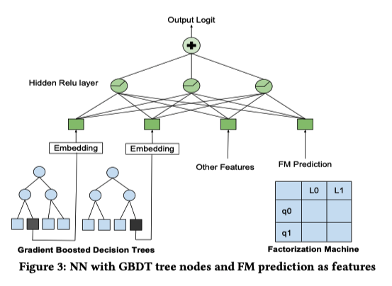
在如何在实时模型中引入 embedding 特征：根据一些规则收集一些 listing，计算这些 listing embedding 的平均值，再和当前排序的 lisitng 计算一个相似度，做为一个特征放到模型中。

如何评估按上面方法生成的 emb sim 特征重要性？利用 GBDT？

[[冷启动]] listing embeddings

• 找方圆 10 英里之内的 3 个最相似的 listing，取 listing embedding 的平均

使用 Embedding 方法要考虑的问题：#card

• 1. 希望Embedding表达什么，即选择哪一种方式构建语料
• 2. 如何让Embedding向量学到东西
• 3. 如何评估向量的效果
• 4. 线上如何使用

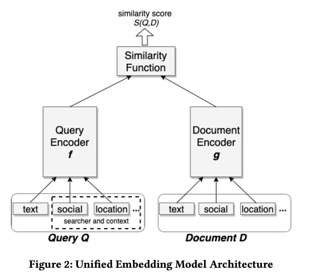
基于 [[向量化召回统一建模框架]] 角度理解

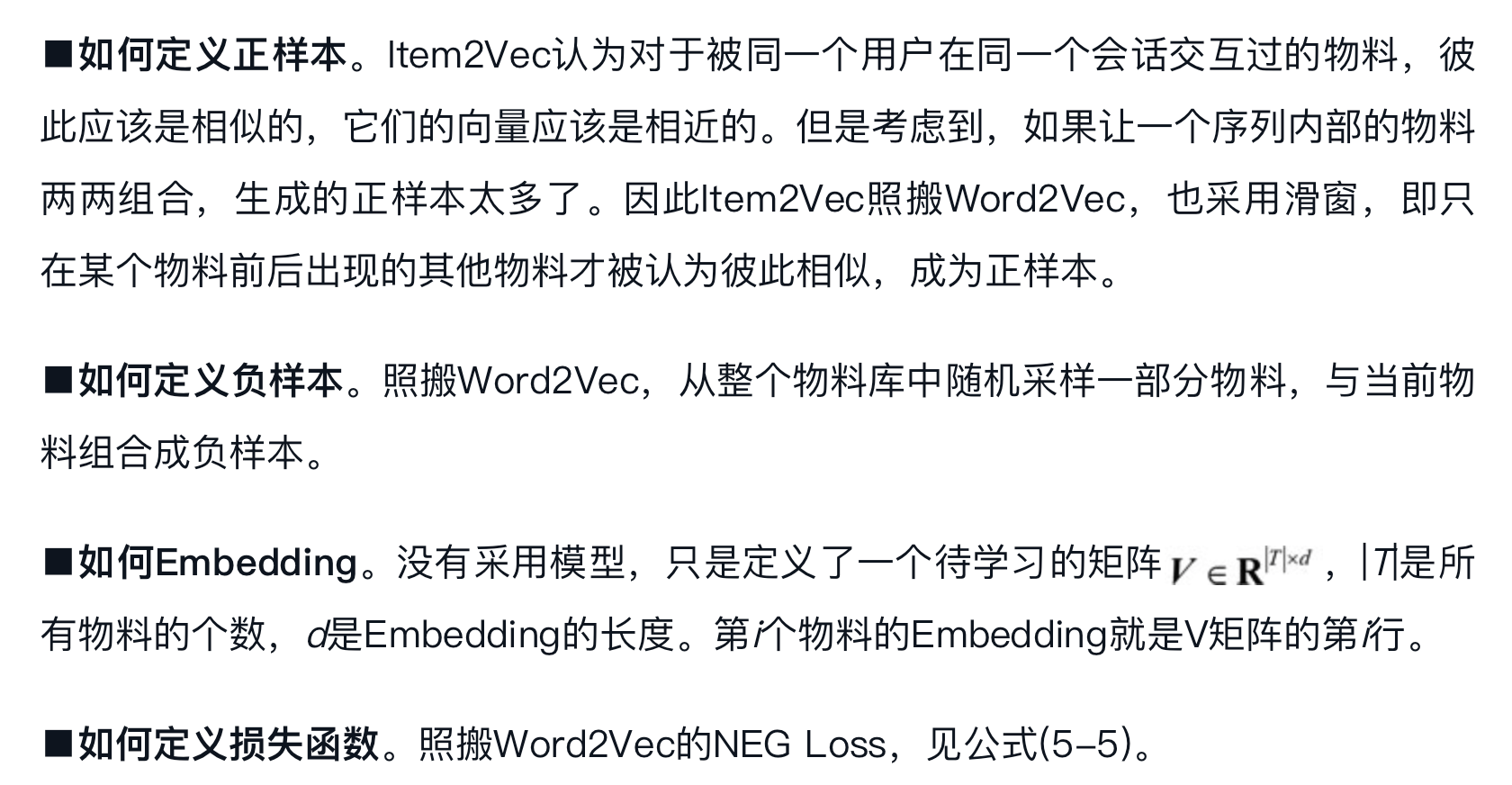
• 如何定义正样本 #card
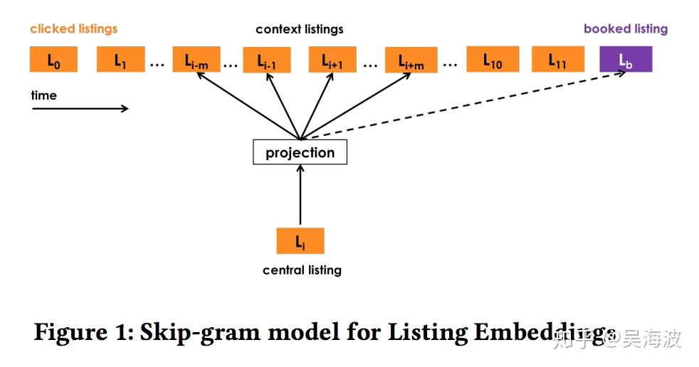
  • 如同前边分析的那样，给定 $t$ 个用户点击的房屋（Airbnb叫 listing）序列，序列内部的房屋，其两两之间都应该是相似的。
  • 但由于两两组合太多，因此仿照Word2Vec采用滑窗，认为某个房屋 I 只与窗口内的有限几个房屋 $c$ 是相似的。
  • 但是，如果一个点击序列最终导致某个房屋 $l_b$ 成功预订，则 $l_b$ 业务信号非常强，必须保留。
  • 因此，Airbnb还额外增加了一批正样本，即点击序列中的每个房屋 I 与最终被成功预订的房屋 $l_b$ 是相似的。
• 如何定义负样本 #card
  • 根据召回的一贯原则，随机采样得到的其他房屋肯定是主力负样本。
  • 但是民宿中介的业务特色决定了，在一个点击序列中的房屋（即正样本）基本上都是同城的，而随机采样得到的负样本多是异地的。
  • 如果只有随机负采样，模型可能只使用“所在城市是否相同”这一粗粒度差异来判断两房屋相似与否，导致最终学到的房屋句量按所在城市聚类，而忽视了同一城市内部不同房屋的差异。
  • 为了弥补随机负采样的不足，Airbnb还为每个房屋在与其同城的其他房屋中采样一部分作Hard Negative， 迫使模型关注所在城市之外的更多细节。
• 如何使用 embedding #card
  
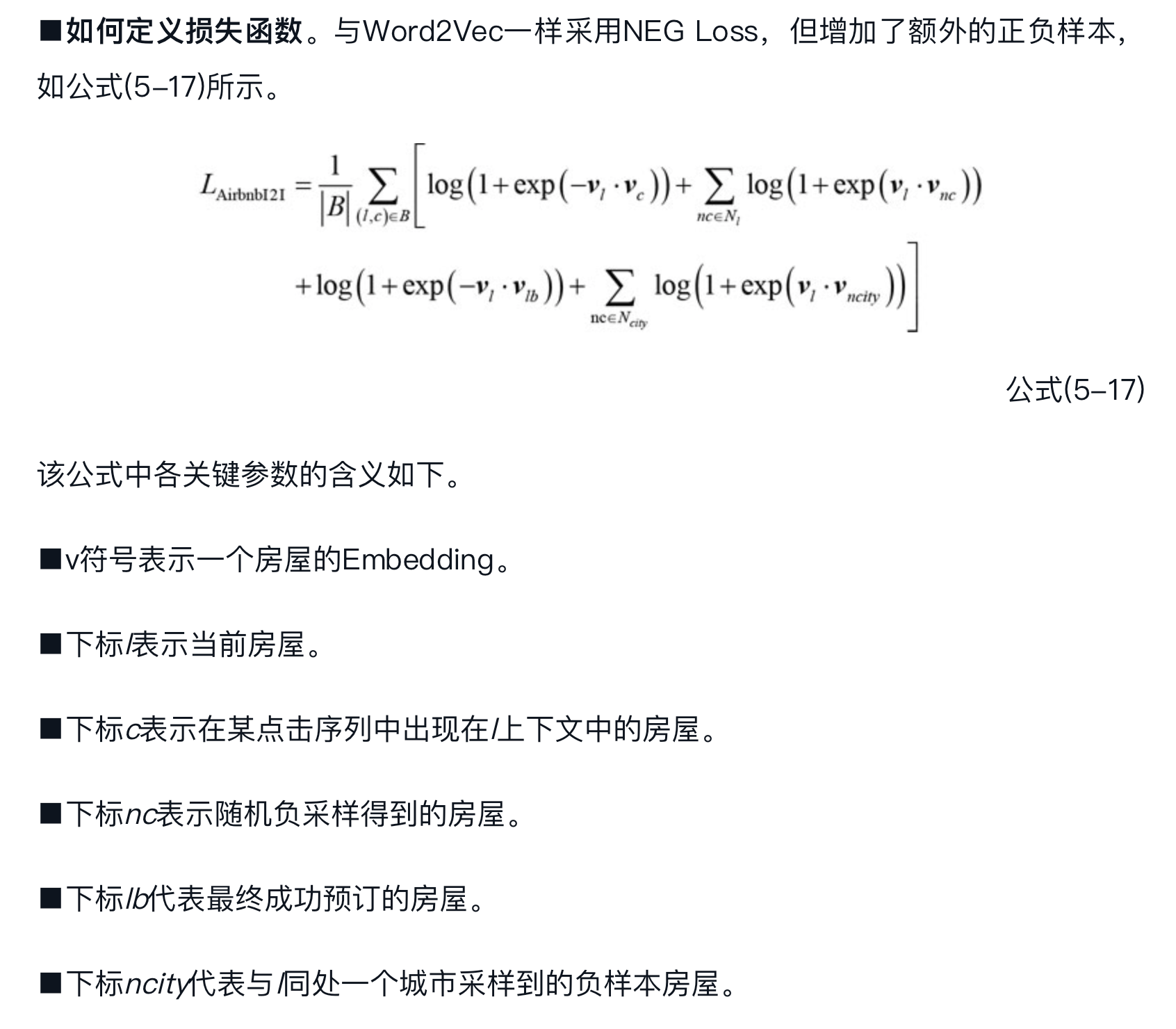
• 如何定义损失函数 #card
  

从[[向量化召回统一建模框架]] 来理解从用户类别到房屋类别的召回

• 如何定义正样本 #card
  
• 如何负样本 #card
  
• 如何 embedding #card
  
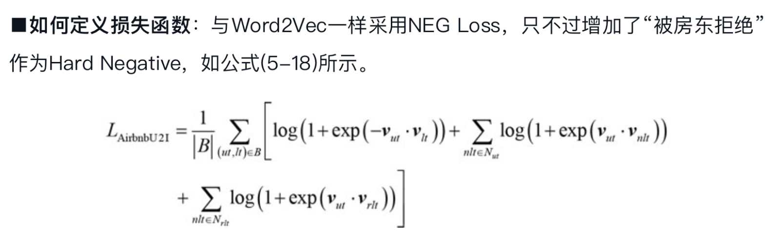
• 如何定义损失函数 #card
  

[[Abstract]]

• CTR prediction in real-world business is a difficult machine learning problem with large scale nonlinear sparse data. In this paper, we introduce an industrial strength solution with model named Large Scale Piece-wise Linear Model (LS-PLM). We formulate the learning problem with L1 and L2,1 regularizers, leading to a non-convex and non-smooth optimization problem. Then, we propose a novel algorithm to solve it efficiently, based on directional derivatives and quasi-Newton method. In addition, we design a distributed system which can run on hundreds of machines parallel and provides us with the industrial scalability. LS-PLM model can capture nonlinear patterns from massive sparse data, saving us from heavy feature engineering jobs. Since 2012, LS-PLM has become the main CTR prediction model in Alibaba’s online display advertising system, serving hundreds of millions users every day.

[[Attachments]]

• Learning Piece-wise Linear Models from Large Scale Data for Ad Click Prediction_2017_Gai.pdf {{zotero-linked-file “attachments:Learning Piece-wise Linear Models from Large Scale Data for Ad Click Prediction_2017_Gai.pdf”}}

分片线性方式对数据进行拟合，将空间分成多个区域，每个区域使用线性的方式进行拟合，最后的输出变为多个子区域预测值的加权平均。

相当于对多个区域做一个 [[Attention]]

结构与三层神经网络类似

Model

处理大规模稀疏非线性特征

LS-PLM 模型学习数据的非线性特征。

question 为什么 LR 模型不能区分下面的数据，如何区分数据？[[SVM]][[FM]]

$$p(y=1 | x)=g\left(\sum_{j=1}^{m} \sigma\left(u_{j}^{T} x\right) \eta\left(w_{j}^{T} x\right)\right)$$

u 和 w 都是 d 维向量

m 为划分 region 数量

一般化使用：

$$p(y=1 | x)=\sum_{i=1}^{m} \frac{\exp \left(u_{i}^{T} x\right)}{\sum_{j=1}^{m} \exp \left(u_{j}^{T} x\right)} \cdot \frac{1}{1+\exp \left(-w_{i}^{T} x\right)}$$

可以把上面的模型看成是三层神经网络

Regularization

• $$\arg \min {\Theta} f(\Theta)=\operatorname{loss}(\Theta)+\lambda|\Theta|{2,1}+\beta|\Theta|_{1}$$
• L1 和常规一样，保持参数的稀疏性。
• L2 如下面的公式，对每一个 feature 的参数进行二阶正则，然后累加。最优化的过程中，L2 项越来越小，相当于做特征选择。每一个特征不止一个参数，只有某一个特征的全部参数都为 0 ，代表这个特征是没有用的。
• $$|\Theta|{2,1}=\sum{i=1}^{d} \sqrt{\sum_{j=1}^{2 m} \theta_{i j}^{2}}$$
• 正则后的效果：
  

@wait 后面如何求解这损失函数以及工程实现待看。

[[Ref]]

• CTR预估 五: Algorithm-LR扩展: MLR - 知乎
• 回顾阿里经典CTR预估模型MLR - 知乎

[[Abstract]]

• Many Collaborative Filtering (CF) algorithms are item-based in the sense that they analyze item-item relations in order to produce item similarities.
• Recently, several works in the field of Natural Language Processing (NLP) suggested to learn a latent representation of words using neural embedding algorithms. Among them, the Skip-gram with Negative Sampling (SGNS), also known as [[Word2Vec]], was shown to provide state-of-the-art results on various linguistics tasks.
• In this paper, we show that item-based CF can be cast in the same framework of neural word embedding.
  • Inspired by SGNS, we describe a method we name item2vec for item-based CF that produces embedding for items in a latent space.
  • The method is capable of inferring item-item relations even when user information is not available.
• We present experimental results that demonstrate the effectiveness of the item2vec method and show it is competitive with SVD.

[[向量化召回统一建模框架]] 理解

• 如何定义正样本。#card
  • Item2Vec认为对于被同一个用户在同一个会话交互过的物料，彼此应该是相似的，它们的向量应该是相近的。
  • 但是考虑到，如果让一个序列内部的物料两两组合，生成的正样本太多了。
  • 因此Item2Vec照搬Word2Vec，也采用滑窗，即只在某个物料前后出现的其他物料才被认为彼此相似，成为正样本。
• 如何定义负样本。#card
  • 照搬Word2Vec，从整个物料库中随机采样一部分物料，与当前物料组合成负样本。
• 如何 embedding #card
  
• 如何定义损失函数 #card
  • word2vec neg loss